Can I use the SUMPRODUCT function with merged cells in Google Sheets?
Yes! It’s possible—similar to how we use SUMIF with merged cells. By virtually unmerging and filling in the arrays used in SUMPRODUCT, we can get accurate results even when the original data includes merged cells.
I’ll walk you through how to do this in Google Sheets.
What Do We Want to Achieve?
The SUMPRODUCT function lets us calculate the sum of products in one go. It also allows us to apply criteria to include or skip certain rows.
For example, in a dataset that contains multiple products such as “ISMC 75”, “ISA 75X75X6”, and “ISMB 200” (common structural steel items), we can use SUMPRODUCT to calculate totals for any one of them—or for all of them.
If we want to target a specific item, we must include a condition in the formula.
Let’s do exactly that in the example below.
But first, here’s what we want to achieve:
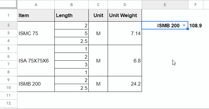
In the dataset, some of the cells in the columns for items, units, and unit weights are merged.
In cell F2, I have a SUMPRODUCT formula that successfully calculates the sum of products, even with merged cells in play.
SUMPRODUCT with Merged Cells in Google Sheets – Example
As I mentioned, some cells in the data range used by the formula are merged.
Despite that, the SUMPRODUCT formula in cell F2 returns the correct product sum based on the selected item in cell E2.
For example, if I select ISMB 200 from the drop-down in cell E2, the formula calculates the result as:
=2*24.2 + 2.5*24.2Before I show you the formula in cell F2, let’s first look at what the formula would be if there were no merged cells in the data range. That will help you understand the necessary adjustments for merged cells.
SUMPRODUCT with Merged Cells in Google Sheets (Formula and Explanation)
Let’s assume we’ve unmerged and reformatted the data like this:
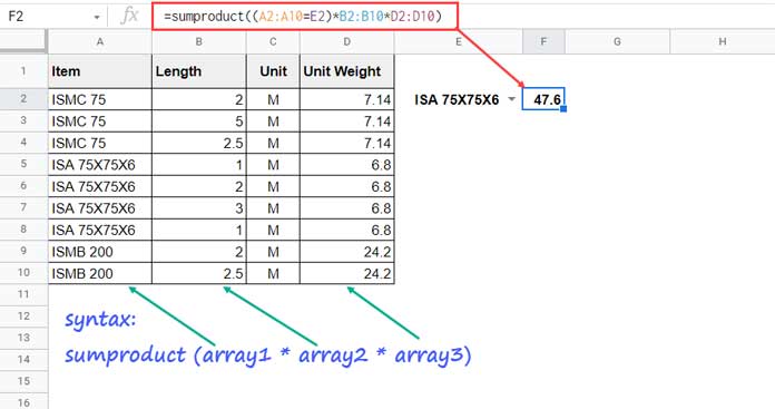
In that case, the formula would be:
=SUMPRODUCT(
  (A2:A10=E2) *
  B2:B10 *
  D2:D10
)
This formula multiplies the quantity (column B) and unit weight (column D) only when the item in column A matches the value in cell E2.
But since columns A and D contain merged cells, we need to virtually unmerge and fill them. That’s where LOOKUP comes in.
Here’s how we generate a virtual unmerged array:
For A2:A10 (items):
LOOKUP(ROW(A2:A10), IF(LEN(A2:A10), ROW(A2:A10)), A2:A10)For D2:D10 (unit weights):
LOOKUP(ROW(A2:A10), IF(LEN(D2:D10), ROW(A2:A10)), D2:D10)These formulas fill down the merged values so SUMPRODUCT can process the arrays properly.
Now, here’s the full SUMPRODUCT formula in cell F2, designed to work with merged cells:
=SUMPRODUCT(
  (LOOKUP(ROW(A2:A10), IF(LEN(A2:A10), ROW(A2:A10)), A2:A10) = E2) *
  B2:B10 *
  LOOKUP(ROW(A2:A10), IF(LEN(D2:D10), ROW(A2:A10)), D2:D10)
)
To better understand the LOOKUP part, see my in-depth tutorial: How to Fill Merged Cells Down or to the Right in Google Sheets
Conclusion
To adapt this formula to a larger dataset or include more columns, simply replace the relevant ranges inside the LOOKUP formulas.
Make sure you update the ranges outside the ROW() function accordingly, while keeping the rest of the logic intact.
That’s all about how to use SUMPRODUCT with merged cells in Google Sheets.
You’ll find a sample sheet and additional resources below to help you work with merged cells more effectively.


