Create a Multi-Column Search Box in Google Sheets

A multi-column search box is a great way to quickly find relevant data in Google Sheets. Instead of searching through individual columns, you can search across multiple columns at once and instantly filter results.

For example, in an employee database, you can search by employee ID, name, department, job title, location, or even email to find the exact information you need.

In this tutorial, I’ll walk you through step by step on how to create a multi-column search box in Google Sheets using a formula-based approach.

A search box like this can be useful for many datasets, including:

Employee records
Material part lists
Purchase orders
Outstanding liabilities
Bills of materials (BOMs)

I’ve implemented word boundaries in this formula to prevent false positives—for example, searching for “oil” won’t match “Foil”, but it will match “Canola oil”. If you prefer partial matching, I’ll show you how to tweak the formula later.

Let’s use an employee database as an example:

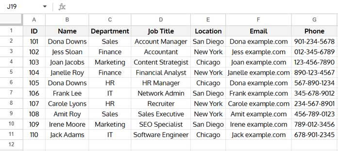
Sample Data for Multi-Column Search Box in Google Sheets

This dataset is stored in Sheet1, and the range is A1:G. When we write the formula, I’ll explain how to adjust it for different data ranges.

You can make a copy of the sample Google Sheet by clicking this link, which will prompt you to create your own editable version.

Go to Sheet2 (or any sheet where you want to place the search box).

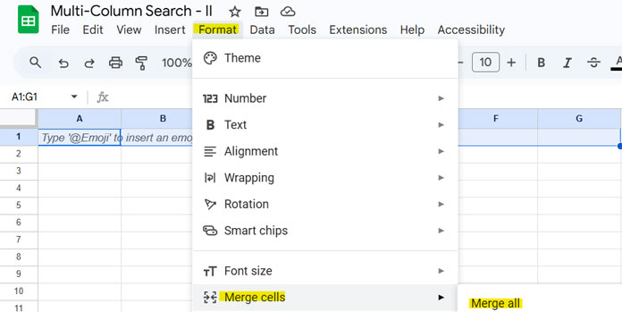
Select cells A1 to G1 and merge them to create a single search field.
- Click Format > Merge cells > Merge all.

Now, cell A1 will serve as the search input box.

Step 2: Formula to Filter Data Based on Search

Paste this formula in A2 of Sheet2 (just below the search box):

=VSTACK(Sheet1!A1:G1, FILTER(Sheet1!A2:G, REGEXMATCH(TRANSPOSE(QUERY(TRANSPOSE(Sheet1!A2:G), , 9^9)), "(?i)\b"&A1&"\b")))

How the Formula Works:

Sheet1!A1:G1 → Keeps the header row intact.
FILTER(Sheet1!A2:G, condition) → Filters only matching rows.
TRANSPOSE(QUERY(TRANSPOSE(Sheet1!A2:G), , 9^9)) → Combines all column values into a single searchable text block per row.
REGEXMATCH(..., "(?i)\b"&A1&"\b") → Matches the exact whole word (case-insensitive).

Now, just type a keyword into A1:

“HR” → Shows all employees in the HR department
“Alice Brown” → Shows Alice’s full details
“New York” → Shows all employees based in New York

Filtering Data Using Multi-Column Search Box in Google Sheets

Note: This formula only matches whole words due to \b. Searching "Soft" won’t return "Software Engineer".

If the search box is left empty, the full dataset remains visible.

Want Partial Matching? (Optional Tweaks)

If you want partial matches (e.g., searching "Soft" should match "Software Engineer"), modify the formula by removing \b:

=VSTACK(Sheet1!A1:G1, FILTER(Sheet1!A2:G, REGEXMATCH(TRANSPOSE(QUERY(TRANSPOSE(Sheet1!A2:G), , 9^9)), "(?i)"&A1)))

Now, searching “Soft” will return “Software Engineer”.

Formula Explanation (Step-by-Step)

1. Transpose Data for Easy Search

TRANSPOSE(Sheet1!A2:G)

Converts rows to columns so that each employee’s details are grouped in a single column.

2. Combine All Column Data Per Row

QUERY(TRANSPOSE(Sheet1!A2:G), , 9^9)

Merges all column values into one cell per row, making it easier to search.

3. Transpose Back to Rows

TRANSPOSE(QUERY(TRANSPOSE(Sheet1!A2:G), , 9^9))

Restores the original row format, but now each row has all of its details merged.

4. Perform the Search

REGEXMATCH(..., "(?i)\b"&A1&"\b")

Matches the exact whole word in any row.

5. Filter and Display Results

FILTER(Sheet1!A2:G, REGEXMATCH(...))

Displays only rows where the search matches.

6. Add Headers with VSTACK

VSTACK(Sheet1!A1:G1, FILTER(...))

Keeps the header row in place.

FAQs (Frequently Asked Questions)

By default, no (because of \b). Searching “Soft” won’t match “Software Engineer”, as the formula looks for whole words only. However, searching “Software” will match “Software Engineer”.

To allow partial matching, remove \b from the formula.

2. Is the search case-sensitive?

No, it’s case-insensitive due to "(?i)". Searching "new york" will match "New York".

3. Can I apply this to a different dataset?

Yes! Simply replace Sheet1!A1:G1 (the header row) and Sheet1!A2:G (the data range) with the corresponding ranges from your dataset.

4. What if I want to search specific columns only?

Update Sheet1!A2:G in the formula to include only the columns you want to search. Make sure to adjust the header row range (Sheet1!A1:G1) accordingly.

Conclusion

A multi-column search box makes it super easy to filter data in Google Sheets without using built-in filters. Whether you’re working with employee records, part lists, or invoices, this method is fast, flexible, and scalable.

If you found this guide helpful, let me know in the comments!

15 COMMENTS

Kardha September 14, 2023 At 6:13 pm

Prashanth,

Thanks for the Search Box tutorial. I’m facing an issue when multiple users open the Google Sheet and enter their desired search text in the search box: the results are not shown.

The search works well when only one user is accessing the sheet, but not when more than one user is accessing the sheet. Is there a way to make the search capabilities work for multiple users at the same time?

Pete December 10, 2020 At 8:38 pm

This works great I have 2600 lines, columns a-n and the only issue is it only displays 10-16 search results, not 2600 if applicable.

- Prashanth December 11, 2020 At 6:20 am
  
  Hi, Pete,
  
  I don’t know what is the issue. Please see the answer to Dave. I’ve provided him a link to another tutorial related to a multi-column search.
  
  If that doesn’t help, if possible, give me access to your sheet. I’ll try to solve the problem.
  
Moni Musial November 21, 2020 At 1:11 am

Thank you for your help. I am trying to create a search bar for work and I have the formula working BUT I am not liking that when the box is empty where I am working I have all the results. Is there a way to get it so that the results only show up when there are works in the search box cell?

- Prashanth November 21, 2020 At 7:16 am
  
  Hi, Moni Musial,
  
  Thanks for your valuable feedback!
  
  Regarding your query, we can do that by using an IF statement that involves Counta.
  
  =if(counta(G1:H2),filter(A2:D,search(G2,B2:B),search(H2,C2:C)),)
  
  This will only work if any of the cells in the criteria fields G1:H2 have any values.
  
  The below formula will only work if there are conditions in G2:H2. Giving only the field labels in G1:H1 is not enough.
  
  =if(counta(G2:H2),filter(A2:D,search(G2,B2:B),search(H2,C2:C)),)
  
Dave September 4, 2020 At 6:28 pm

Hoping you still monitor this.

I have about 7 columns I want to do Filter and Search across, but it seems the more search boxes I add, the more problems I get with the results, in that a number of results are missing.

Does filter + search have known limitations like this, or if several search boxes are empty, it breaks down?

- Prashanth September 5, 2020 At 9:31 am
  
  Hi, Dave,
  
  I’ve once again gone through the tutorial.
  
  I haven’t found any issue in the formula. But I have noticed one thing, i.e. you can leave any criteria field blank. But entering a criterion that’s not available in the corresponding column makes the formula breaks!
  
  To avoid that use the data validation drop-box in the search fields. So you can select a valid criterion.
  
  If you still have issues with the formula, please leave the URL of your sheet in the reply (which I won’t publish). So that I can have a look.
  
  In addition to the above, there is one more multi-column search box tutorial – Filter Rows if Search Key Present in Any Cell in that Rows in Google Sheets.
  
TYSON November 13, 2019 At 12:49 pm

Keep up the good work Prashanth and thank you. I have adapted formula for 10 columns and made my life so much easier.

Amazing how little tricks make a massive difference.

Cheers

- Tammy November 14, 2019 At 2:14 pm
  
  How did you do that? When I more than 3 “search functions” within the filter(), I get an error that says:
  
  ERROR: FILTER RANGE must be a single row or column
  
Matt Larrubia October 24, 2019 At 10:49 pm

Hi,

I currently created a google form that has the following fields: User, Period, lab, URL.

I want to create a function that will allow me to filter into a NEW spreadsheet that holds all the users’ labs. So essentially I can view all the Labs from a User dynamically as they fill out the form.

So if the user submits the form with a new lab it will add another column to their row. Can you suggest any articles/videos help me accomplish this?

Thank you in advance.

- Prashanth October 25, 2019 At 1:56 pm
  
  Hi, Matt,
  
  Can you share the screenshot/or Sheet itself of your user-submitted data (sample) and the result you want?
  
  Best,
  
Josh June 3, 2019 At 6:21 am

Hi,

I’m trying to use the filter function but with a universal lookup value.

Example: If A1 contains the lookup value then something like the following:

=filter(C:C,D:D=$A$1,)OR(filter(C:C,E:E=$A$1,)

At the moment I have the lookup value for different columns in different cells running an ‘if’ function. Check A1, if blank check A2, if blank check A3, etc.

Any ideas on this?
Thanks in advance!
Josh

- Prashanth June 3, 2019 At 8:17 am
  
  Hi, Josh,
  
  I wish to see a demo sheet with the above problem to give an answer.
  
PETIT C January 19, 2019 At 6:25 pm

Hi,

Does it work with a regex formula if you wish to find a single word in multiple columns?

- Prashanth January 20, 2019 At 12:31 pm
  
  Hi,
  
  Please provide more details.
  
  Best,