In VLOOKUP, you can skip blank cells in the result (index) column and continue looking up the search key in Google Sheets. To achieve this, you can use either the FILTER function or the QUERY function in combination with VLOOKUP.

VLOOKUP searches down the first column in a range for your given search key. If found, the formula returns the value from the corresponding cell in the specified column of that row. You might already know this.

The returned cell value can be any type (text, numeric, or date) and may sometimes be blank. If the cell is blank, VLOOKUP does not skip the row and continue searching for the next available value. Instead, it returns a blank result.

For example, suppose my search key is “Pebbles”. I want a VLOOKUP formula that searches down column A in the range A2:D for the value “Pebbles” and returns the value from the same row in column C. Using VLOOKUP in this case, it would return a blank.

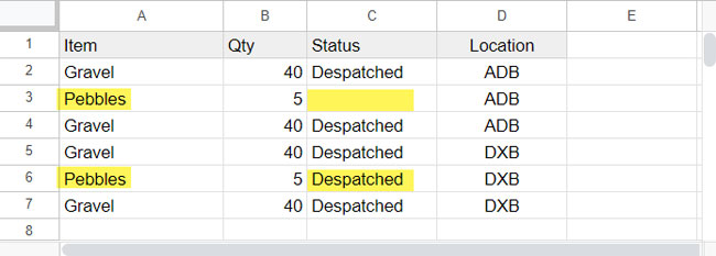
=VLOOKUP("Pebbles", A2:D, 3, FALSE)

As you can see, VLOOKUP finds the search key “Pebbles” in cell A3. We want the result from column C in that row, which is the value in cell C3.

Since cell C3 is blank, VLOOKUP will only return a blank. To skip this row and search for the second occurrence of “Pebbles” in column A (i.e., cell A6), and return the value from cell C6, which is not blank, you can use the following approach.

Step 1: Filter Out Blank Rows Based on Index Column

VLOOKUP uses the column index to return a value where the first column in the ‘range’ is numbered 1.

VLOOKUP(search_key, range, index, [is_sorted])

If you want to return a value from the third column, you should filter the range based on a condition applied to column 3.

To filter out blank rows, you can use the following formulas:

Using the FILTER function:

=LET(range, A2:D, FILTER(range, CHOOSECOLS(range, 3)<>""))

Where:

• A2:D is the range.
• 3 is the index for the third column.

Using the QUERY function:

=LET(range, A2:D, QUERY(range, "SELECT * WHERE Col3 IS NOT NULL"))

Where:

• A2:D is the range.
• Col3 refers to the index of the third column.

You can use one of these formulas as the range in VLOOKUP to skip blank cells in the results.

When using it, replace A2:D with your lookup range and 3 or Col3 with the index number of the result column.

Step 2: Skip Blank Cells and Continue Search in VLOOKUP

Now it’s easy. Use either the QUERY or FILTER function as a virtual range within VLOOKUP. The rest of the arguments will remain the same.

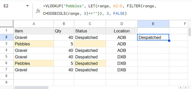
Example Using FILTER Range:

=VLOOKUP("Pebbles", LET(range, A2:D, FILTER(range, CHOOSECOLS(range, 3)<>"")), 3, FALSE)

• search_key: “Pebbles”
• range: LET(range, A2:D, FILTER(range, CHOOSECOLS(range, 3)<>””))
• index: 3
• is_sorted: FALSE

Example Using QUERY Range:

=VLOOKUP("Pebbles", LET(range, A2:D, QUERY(range, "SELECT * WHERE Col3 IS NOT NULL")), 3, FALSE)

• search_key: “Pebbles”
• range: LET(range, A2:D, QUERY(range, “SELECT * WHERE Col3 IS NOT NULL”))
• index: 3
• is_sorted: FALSE

This is how you skip blank cells in the result column and continue searching for the key with VLOOKUP.

Possible Errors and Troubleshooting:

The VLOOKUP and FILTER or QUERY combination will return #N/A errors in two cases:

• When the search key is not present in the lookup range.
• When the index column contains only empty cells.

To handle these errors, you can wrap the formulas with IFNA to remove #N/A errors. The formulas would be as follows:

=IFNA(VLOOKUP("Pebbles", LET(range, A2:D, FILTER(range, CHOOSECOLS(range, 3)<>"")), 3, FALSE))
=IFNA(VLOOKUP("Pebbles", LET(range, A2:D, QUERY(range, "SELECT * WHERE Col3 IS NOT NULL")), 3, FALSE))

Using INDEX-MATCH to Skip Blank Cells in VLOOKUP Results

If you’re looking for an alternative solution to handle blank cells in VLOOKUP results, you can use the INDEX and MATCH combination:

=INDEX(C2:C, MATCH(1, (A2:A="Pebbles")*(C2:C<>""), FALSE))

Here’s a breakdown of how this formula works:

• (A2:A= "Pebbles"): Returns TRUE where the Item column matches the search key “Pebbles”.
• (C2:C<> ""): Returns TRUE where the Status column is non-empty.
• (A2:A= "Pebbles") * (C2:C<> ""): Multiplies these two conditions. This returns 1 wherever the search key matches in column A and the corresponding cell in column C is not empty (TRUE * TRUE = 1).

The MATCH function finds the position of 1 in the resulting array:

MATCH(1, ..., FALSE)

Finally, the INDEX function returns the value from the Status column based on the position provided by MATCH:

INDEX(C2:C, MATCH(1, ..., FALSE))

This approach allows you to skip blank cells in the result column if you are less familiar with using FILTER or QUERY functions.

Resources

• Move the Index Column If Blank in VLOOKUP in Google Sheets
• VLOOKUP to Get the Last Non-blank Value in a Row in Google Sheets