Dynamic column references in QUERY can be based on matching header labels or using a sequence of numbers, rather than hardcoding column letters.
For matching column labels, you can use XMATCH. For selecting a sequence of columns from one point to another, you can use the SEQUENCE function.
In both cases, you might also need to use TEXTJOIN and ARRAYFORMULA. This tutorial may be helpful for these advanced techniques.
To identify columns in the SELECT clause of a QUERY, you can use either column letters (like A, B, C) or column numbers (like Col1, Col2, Col3). Since XMATCH and SEQUENCE return column numbers, using column numbers in your QUERY is often more convenient. These functions or calculations determine the column number at runtime.
👉 For an overview of all dynamic column selection methods in Google Sheets QUERY, refer to the main hub post.
Dynamic Column References in QUERY Using the SEQUENCE Function
This technique is useful for selecting columns in QUERY from one point to another. For example, in a data range with 25 columns, you can select columns from n_1 to n_2, where n_1 and n_2 are numbers from 1 to 25, with n_2 being greater than or equal to n_1. For instance, to get columns from 11 to 20, set n_1 to 11 and n_2 to 20.
Here’s how to dynamically refer to columns in QUERY using SEQUENCE.
Enter the following sample data in Sheet1 in your Google Sheets file:
| Date | Sales | Returns | Net Sales |
| 2024-01-01 | 100 | 5 | 95 |
| 2024-01-02 | 150 | 10 | 140 |
| 2024-01-03 | 200 | 15 | 185 |
| 2024-01-04 | 120 | 7 | 113 |
| 2024-01-05 | 180 | 8 | 172 |
Normally, you might use the following formula in cell A1 in Sheet2 to select columns 1 to 4:
=QUERY(
   Sheet1!A1:D,
   "SELECT Col1, Col2, Col3, Col4 WHERE Col1 IS NOT NULL",
   1
)
This returns columns 1 to 4 from the data and filters out rows where column 1 is empty.
When dealing with a larger range, such as 50 columns, manually specifying column numbers becomes impractical. Here’s where dynamic column references using SEQUENCE come in handy.
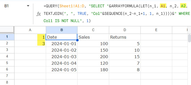
To dynamically select columns, enter the following formula in cell B1 in Sheet2:
=QUERY(
   Sheet1!A1:D,
   "SELECT "&ARRAYFORMULA(LET(n_1, 1, n_2, 4, TEXTJOIN(", ", TRUE, "Col"&SEQUENCE(n_2-n_1+1, 1, n_1))))&" WHERE Col1 IS NOT NULL",
   1
)
In this formula, n_1 is 1 and n_2 is 4, and they are hardcoded. If you wish, you can enter them in two cells and refer to those:
Example:
=QUERY(
   Sheet1!A1:D,
   "SELECT "&ARRAYFORMULA(LET(n_1, A1, n_2, A2, TEXTJOIN(", ", TRUE, "Col"&SEQUENCE(n_2-n_1+1, 1, n_1))))&" WHERE Col1 IS NOT NULL",
   1
)
For a data range of A1:Z and columns 11 to 20, enter 11 in A1 and 20 in A2.
This approach dynamically adjusts the columns selected based on the specified range.
SEQUENCE Part Breakdown
(You can skip this formula explanation if you prefer.)
Syntax:
SEQUENCE(rows, [columns], [start], [step])Formula Part:
SEQUENCE(n_2-n_1+1, 1, n_1)rows:n_2-n_1+1columns:1start:n_1
If n_1 is 11 and n_2 is 20:
rowswill be 10 (20−11+1=10)columnswill be 1startwill be 11
So the SEQUENCE function returns the numbers 11 to 20.
With each number, we combine the text “Col” and then use TEXTJOIN to join them, using a comma separator.
TEXTJOIN(", ", TRUE, "Col"&SEQUENCE(n_2-n_1+1, 1, n_1))The LET function is used to assign the names n_1 and n_2, and the ARRAYFORMULA is used because the concatenation of “Col” in an array requires it.
Common Errors & Troubleshooting
Here are the two common errors you may encounter when using dynamic column references with the SEQUENCE function in Google Sheets:
- #NUM – This error occurs when
n_2is smaller thann_1 - #VALUE – This error occurs when the number of columns is larger than the available number of columns in the data.
To troubleshoot, correct n_1 and n_2 values.
If you are already using IFERROR with QUERY, you won’t see these errors. Therefore, I don’t suggest using IFERROR with QUERY in this case.
Additional Tips
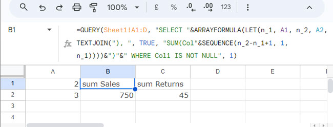
Instead of selecting columns, if you want to aggregate all columns, you can use the following formula:
SELECT "&ARRAYFORMULA(LET(n_1, A1, n_2, A2, TEXTJOIN("), ", TRUE, "SUM(Col"&SEQUENCE(n_2-n_1+1, 1, n_1))))&")"&"Enter n_1 in cell A1 and n_2 in cell A2. Make sure that all selected columns are numeric.
In this formula, you can replace SUM with AVERAGE, COUNT, MIN, or MAX aggregation functions in QUERY.
Dynamic Column References in QUERY Using the XMATCH Function
This is useful when you want to use QUERY to select columns based on a list of column names (field labels) specified in a list.
In our sample data in A1:D (Sheet1), the field labels are Date, Sales, Returns, and Net Sales.
The QUERY function doesn’t support using these column names in the formula instead of column letters.
To achieve this, enter the field labels in a column and use QUERY to dynamically refer to and select the columns based on the column names in the provided list, in that order.
In Sheet2, enter the field labels that you want to dynamically refer to in the QUERY formula. For example, enter Date, Sales, and Returns in cell range A1:A.
Enter the following formula in cell C1 in that sheet:
=QUERY(Sheet1!A1:D, "SELECT "&TEXTJOIN(", ", TRUE, ARRAYFORMULA("Col"&XMATCH(TOCOL(A1:A, 1), Sheet1!A1:D1)))&" WHERE Col1 IS NOT NULL", 1)
Where:
A1:Ais the list reference.Sheet1!A1:D1is the header row reference in the data.
The XMATCH function matches the column names in the list to the header row and returns their relative positions in the list. We have specified the list as TOCOL(A1:A, 1) instead of A1:A because TOCOL removes blank cells in the list range.
As earlier, we combine the string “Col” with the positions and join the numbers using TEXTJOIN.
Error Handling:
This formula may return VALUE errors in the following cases:
- If the list is empty
- If the list contains repeated column names
If one of the list items doesn’t match the header, the formula may return the #N/A error.
When using the XMATCH approach to get dynamic column references, it’s advisable to wrap the QUERY with the IFERROR function.
Example:
=IFERROR(QUERY(
   Sheet1!A1:D,
   "SELECT "&TEXTJOIN(", ", TRUE, ARRAYFORMULA("Col"&XMATCH(TOCOL(A1:A, 1), Sheet1!A1:D1)))&" WHERE Col1 IS NOT NULL",
   1
))


Thanks for this. Is there a way to add a WHERE clause that queries the same dynamic column we found in the first part of the query?
As opposed to the “ColX” format, as per the comments above.
Hi, Arif I,
Sorry, I couldn’t understand. I suggest you share a sample sheet (URL) with more info via the comment below.
Could you please help explain why we need to put the curly brackets
{A1:M5}in the query instead ofA1:M5?Hi, An Dang,
The difference is in the use of column identifiers.
There are two types of column identifiers.
Example:-
Data Range: X1:Z100.
The first column in this range is column X.
You can refer to this column as below (column identifier type 1).
"Select XIt’s the first column in the range X1:Z100.
To refer to that column as (column identifier type 2);
"Select Col1We must make the range, i.e., X1:Z100, an expression. There comes the use of the Curly Brackets.
It works!
Only for me I replaced the original formula and user helper cells so I can re-arrange the order of the columns, and exclude columns I don’t want:
=QUERY({J1:Z14},"Select "&ArrayFormula(textjoin(", ",1,A3:I3)))where row A1 to I1 has helper cells, with the formula
=iferror("Col"&index(Match("*"&A2&"*", $J$2:$Z$2,0)),"")A2 etc, refer to keywords that I want to find out of table headers, as the tables are not consistent in labels, but in content.
Hi Prashanth —
I really appreciate this post it’s very helpful. Can you help me diagnose the formula parse error when I add “where” to my query?
=QUERY({A7:DN130},"Select "&ArrayFormula(textjoin(", ",TRUE,("Col"&row(indirect("A"&41&":A"&118)))) where Col7 = '"&$G167&"'))Hi, Peter Gassiraro,
Let me make you understand by taking one of the formulas from my above tutorial.
=QUERY({A1:M5},"Select "&ArrayFormula(textjoin(", ",TRUE,("Col"&row(indirect("A"&C9&":A"&F9))))))In this the QUERY dynamic column reference formula, if you remove the variables from within the INDIRECT part, it should be something like this.
=QUERY({A1:M5},"Select "&ArrayFormula(textjoin(", ",TRUE,("Col"&row(indirect("A5:A12"))))))To include the WHERE clause, you can follow the below formula.
=QUERY({A1:M5},"Select "&ArrayFormula(textjoin(", ",TRUE,("Col"&row(indirect("A5:A12")))))&" where Col10=255")The formula part
Col10=255should be changed based on the criteria type (text/number/date) which you can find in my corresponding tutorial below.Examples to the Use of Literals in Query in Google Sheets.
So I’m trying to use the same principle on a Where clause using the match function, but it won’t work. What am I missing here?
Formula:
=query({A:K},"Select Col1 where "&"Col"&(match($M$5,$A$2:$K$2,0))='N' and "&"Col"&(match($N$5,$A$2:$K$2,0))='Y'")Hi, J,
Here is the correct way of using the MATCH function in the QUERY WHERE clause.
=query({A:K},"Select Col1 where Col"&MATCH($M$5,$A$2:$K$2,0)&"='N' and Col"&MATCH($N$5,$A$2:$K$2,0)&"='Y'",1)Also, I recommend to use the correct range like A2:K instead of A:K in Query.
Hello,
Any idea how to get a dynamic formula for an importrange sheet selection?
Here is the related guide – Dynamic Sheet Names in Importrange in Google Sheets.
How would you add a where clause to this?
Good question!
Use ampersand to join the Query ‘WHERE’ clause as a text string (within double-quotes).
Example:
=QUERY({A1:M5},"Select "&ArrayFormula(textjoin(", ",TRUE,("Col"&row(indirect("A"&C9&":A"&F9)))))&" where Col1='Apple'",1)Good day,
What will be the formula if it to be liked this,
Instead of
Col5toCol12I need only
Col5andCol12Hi, Austria,
Normally we can use the Query as
=query({A1:E},"Select Col1,Col5")or=query(A1:E,"Select A,E")To refer these two columns dynamically, use the Query as below.
=query({A1:E},"Select Col"&F1&",Col"&G1)In this, the cell F1 contains the number 1 and G1 contains the number 5.
Best,
Another question,
If I specified Col10 and Col15 instead of listing each column how can I change the formula if I just want to see the sum from Col10 to Col15?
Hi, Austria,
Just replace the
,delimiter in the Textjoin to a+.Eg.
The data range is A1:M5 and the first row contains column names.
The value in cell C9 is 2 (indicates the second column and F9 is 5 (indicates the fifth column).
The formula to sum column 2 to 5 is;
In cell O1
=QUERY({A1:M5},"Select "&ArrayFormula(textjoin("+ ",TRUE,("Col"&row(indirect("A"&C9&":A"&F9))))))The cleaner coding of this formula is;
=query({A1:M5},"Select Col2+Col3+Col4+Col5")Actually, you can use MMULT for this. See that detail here – Array Formula to Sum Multiple Columns in Google Sheets and Grouping.
This too – Sum Multiple Columns Dynamically Across Rows in Google Sheets.
Does this dynamic column-selection actually work any more? I just get “NO_COLUMN: Col1” no matter what I try…
Hi, Oliver Steadman,
It works 🙂
I am also unable to use ‘Col#’ instead of A, B, C, etc.
Hi, Ken Lee,
The Query ‘data’ should be within open and clause Curly Brackets or an expression.
QUERY(data, query, [headers])Eg.
=query({A1:F},"Select Col1,Col2")I’ve explained the same within the tutorial.
Thank you — didn’t see that in the tutorial.