Is there an Array Formula to Sum multiple columns in Google Sheets?
I’ve data in hundreds of rows and several columns in one of my Google sheets files.
I want to get the total of columns in each row (row-wise).
I only want to use a single expanding array formula.
The function SUM may not yield expanded results even if you use the function ArrayFormula with it.
You can use the MMULT to get expanded SUM in Google Sheets. With this approach, a single formula can sum the total of columns in each row.
I believe I should make it clearer to you before going into more in-depth details or further elaborating on this topic.
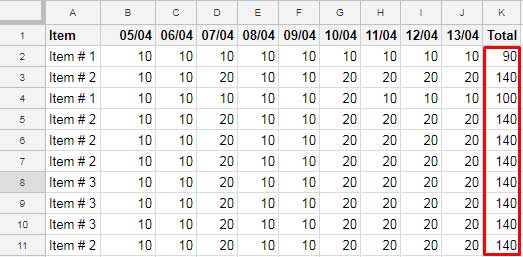
See the below screenshot to understand what I have been talking about.

I am talking about column K, the sum of columns B to J. It’s a row-wise total.
K2 contains the total of the column range B2:J2.
The normal or, you can say, non-expanding sum formula for cell K2 will be as below.
=sum(B2:J2)Even if you use the Array Formula, the Sum formula in K2 can’t expand to the rows below.
=arrayformula(sum(B2:J2))In the above example, there are a limited number of rows.
So you can think about copying and pasting the above non-array sum formula into the cell range K3:K11.
But when the table has hundreds of rows, it’s advisable to use an Array Formula in one cell that automatically expands.
If we use an array formula to sum each row as per the example above, it would be in cell K2.
This post reveals how to get an expanded sum in Google Sheets using an Array Formula.
Array Formula to Sum Multiple Columns in Google sheets
The MMULT function is probably the best way to get expanding sum in Google Sheets. But it’s not the one and only solution.
Here is one regular formula that can be used as an Array Formula to Sum Multiple Columns in Google sheets.
Array Formula 1:
=ArrayFormula(B2:B11+C2:C11+D2:D11+E2:E11+F2:F11+G2:G11+H2:H11+I2:I11+J2:J11)I am skipping the explanation part of this formula as it’s pretty simple to understand. It totals each column and produces an expanding result.
Here I can point out the two main limitations of this formula.
If the number of columns is more, entering the formula is tough without making typos. It’s like a chain of alphabets.
If there are more than 10-20 columns, you will find it tough to enter this formula without any mistakes.
Another problem is its issue with newly inserted columns.
If you insert a new column or columns, you should change the formula to incorporate them. That means it is not a flexible solution.
Let’s code the flexible Array Formula to Sum multiple columns in Google Sheets.
Flexible Array Formula to Sum Multiple Columns in Google sheets
As I’ve mentioned above, I’m using MMULT instead of SUM.
Array Formula 2:
=ArrayFormula(MMULT(n(B2:J11),(transpose(COLUMN(B1:J1)^0))))I’ve already detailed the MMULT formula usage earlier.
Pick this formula (MMULT) topic from my Google Sheets Function Guide to master it.
For a quick reference, here is the syntax of the MMULT function.
MMULT(matrix1, matrix2)Now here is my Array Formula 2 explanation.
The purpose of MMULT is to calculate the matrix product of two matrices. But what we want is Sum.
In my Google Sheets MMULT array formula above (Array Formula 2), the cell range n(B2:J11) is my matrix1.
The N function converts blank cells in the range and returns 0 (zero). Otherwise, MMULT may return an error.
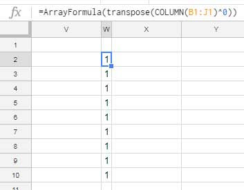
Generate a virtual column for matrix2 that contains only # 1. So there is no effect of the multiplication in MMULT.
I’ve used the Column function to generate the matrix2.

Matrix1 has nine columns from B to J. So, here, matrix2 has nine rows which validate the core matrix multiplication standard as;
the number of columns for matrix1 must equal the number of rows for matrix2
That’s it! Now we are going to the second part of this tutorial.
You can learn here how to Sum multiple columns and group them.
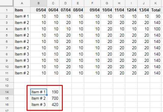
First, see the output of the grouped some marked in the below image.

Here are the steps.
Grouping Part
We can use the above MMULT in Query as the range to get the group-wise sum of multiple columns in Google Sheets.
Formula 3:
=QUERY({A2:A11,ArrayFormula(MMULT(n(B2:J11),(transpose(COLUMN(B1:J1)^0))))},"Select Col1, Sum (Col2) group by Col1 label Sum(Col2)''")In the above formula, the Query range is the above Array Formula 2 (the formula within the Curly Brackets that except the A2:A11 range)
This query formula has two columns.
One is column A2:A11 (please see the sample data on the above screenshot) which contains the names we want to group.
The second column is the above MMULT formula result (the row-wise sum of the range B2:J11).
I’ve joined both these two columns by using the Curly Braces to make a two-column array as below.

In this, as I’ve already said above, column 2 is the combined sum of the range B2:J11.
We can easily group and total these two column ranges in Query.
That’s what I did in the above formula (Formula 3).
Conclusion
You can tweak the above MMULT a little bit to get array results in Count.
I’ve explained that separately.
Similar: How to Expand Count Results in Google Sheets Like Array Formula Does
Learning MMULT is a little complicated. But once you’ve tamed it, you have a function in your hand to manipulate your data effectively in Google Sheets.


Hi Prashanth,
That worked beautifully! Thank you so much!
Is there a way to apply this technique if the first matrix has a varying length for each row? For example, I have a delimited list in column M, where I must split the list, get the value of the leftmost characters up to the first space, and add those values together so that I have a total for each row.
This formula gets me the split results, but I am stuck on how to get a total for each row’s resulting array using a single array formula at the top of my sheet.
=ARRAYFORMULA(IFERROR(VALUE(LEFT(TRIM(SPLIT(M2:M, ",")),FIND(" ", TRIM(SPLIT(M2:M, ",")))-1))))
Example: M2 = “2.50 This is a test, .50 Here is another item, .25 My 3rd selection” and the corresponding total is 3.25
M3 = “2.50 XYZ, .50 ABC” and the corresponding total is 3.
Hi Amy,
I believe you are familiar with LAMBDA functions. You can use the BYROW LAMBDA to solve this.
I am currently updating my old posts. There are over 1,200 of them, so it may take some time.
Here is my proposed formula:
=ARRAYFORMULA(LET(result,BYROW(IFERROR(VALUE(LEFT(TRIM(SPLIT(M2:M, ",")), FIND(" ", TRIM(SPLIT(M2:M, ",")))-1))),
LAMBDA(r,sum(r))),IF(result=0,,result)))
Is there a way to do this without specifying the number of rows?
Hi, Robert.
I guess you were talking about replacing B2:J11 with B2:J in the below formula.
=ArrayFormula(MMULT(B2:J11,(transpose(COLUMN(B1:J1)^0))))If so, try this.
=ArrayFormula(iferror(((1/MMULT(n(B2:J),(transpose(COLUMN(B1:J1)^0))))^-1)))Another way in the above example could be;
=ArrayFormula(MMULT(N(B2:J12), SEQUENCE(COLUMNS(B:J),1,1,0)))A similar one.
=MMULT(D99:J114, transpose(SPLIT(REPT("1,",COLUMNS(D99:J99)),",")))