Need to total values across several columns for each row—without writing a formula in every row? In this tutorial, you’ll learn how to sum multiple columns dynamically in Google Sheets, row by row, using powerful functions like BYROW, LET, and QUERY. Whether your columns are fixed or vary over time, these techniques will help you automate row-wise summing with ease.
You’ll be able to define which columns to include in the sum, either by their column numbers or by their header names.
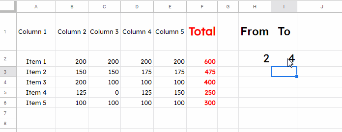
Sum Multiple Columns Dynamically Based on Start and End Columns
In the following example, the data is in range A1:E, and the start and end columns for the sum are specified in cells H2 and I2.
You can use several functions to sum multiple columns dynamically in Google Sheets, including BYROW, QUERY, MMULT, and DSUM. In this tutorial, we’ll focus on the two most effective approaches: QUERY and BYROW.
Using QUERY
=LET(
  cols, ARRAYFORMULA(TEXTJOIN("+", TRUE, "Col"&SEQUENCE(I2-H2+1, 1, H2))),
  QUERY(A1:E, "SELECT "&cols&" LABEL "&cols&" 'Total'")
)
Insert this formula in cell F1, in the header row, to display the total next to each row.
How this formula works:
SEQUENCE(I2-H2+1, 1, H2)generates a list of column numbers (e.g., 2, 3, 4)."Col"&...converts them into QUERY-friendly column references likeCol2,Col3, etc.TEXTJOIN("+", TRUE, ...)combines those into a single string:"Col2+Col3+Col4".QUERYthen adds these columns row-wise and labels the output as “Total”.
Simplified QUERY Version:
=LET(cols, "Col2+Col3+Col4", QUERY(A1:E, "SELECT "&cols&" LABEL "&cols&" 'Total'"))Important: If any cell within the specified columns is blank, the QUERY function will skip that entire row when summing.
Using BYROW (Modern Approach)
=ArrayFormula(
  LET(
    calc, BYROW(
      CHOOSECOLS(A2:E, SEQUENCE(I2-H2+1, 1, H2)),
      LAMBDA(r, SUM(r))
    ),
    VSTACK("Total", IF(calc=0,,calc))
  )
)
What this does:
SEQUENCE(I2-H2+1, 1, H2)builds the list of column indices.CHOOSECOLS(A2:E, ...)selects only those columns.BYROW(..., LAMBDA(r, SUM(r)))sums each row across those selected columns.VSTACK("Total", ...)adds a header label on top.
This is a robust and flexible way to sum multiple columns dynamically in Google Sheets row by row—especially if you’re dealing with modern Sheets features.
Sum Multiple Columns Dynamically Based on Headers
You can also sum columns dynamically using header names instead of column numbers—and the best part is, you don’t need to change the formula at all.
Here’s what to do:
- In cell
H2, enter:=XMATCH("header1", A1:E1) - In cell
I2, enter:=XMATCH("header2", A1:E1)
Replace "header1" and "header2" with your actual column header names (e.g., "Q1", "Q3").
These two formulas will return the start and end column positions dynamically, which plug directly into the formulas shown above. This way, you can sum columns based on header names without editing your sum formula.
Resources
- How to Sum Each Row in Google Sheets– Covers all possible solutions to sum across multiple columns row-wise, including manual methods,
BYROW,MMULT,QUERY, and more. - Array Formula to Sum Multiple Columns in Google Sheets – Use an array formula to sum multiple columns and optionally include or exclude specific columns by header.
- Multiple Sum Columns in SUMIF in Google Sheets
- Dynamic Column References in Google Sheets Query
- Get Last 7, 30, and 60 Days Total in Each Row (from Today) in Google Sheets


I’m wondering which one is faster for this use case in a larger dataset, this Query, or a variation of DSUM?
Hi, Alda,
I would prefer DSUM.