If the index column is blank, the VLOOKUP function will return an empty cell in Google Sheets. How can you retrieve the next non-blank value?

I’m referring to moving or shifting the index column in the VLOOKUP formula when the result is blank. This is a common dilemma faced by VLOOKUP users, whether they’re using Google Sheets or Excel.

Even if the search key is present in the lookup range, VLOOKUP may return a blank result. This can happen if there is no value to return in the corresponding cell of the found row.

Understanding the Problem

For example, I want to return a value from column 2 in the range, so I specify index number 2 in the VLOOKUP formula. However, if the corresponding cell in column 2 is blank, I want to get the value from column 3. If column 3 is also blank, then I want to pull the value from column 4, and so on.

I don’t want to manually change the index number in the VLOOKUP formula (e.g., changing from 3 to 4 to get the value from the fourth column). How can I automate this process?

You might consider searching for the key and returning all the values in the found row using a sequence of index numbers and entering the formula as an array formula. But that only partially solves the problem. You want the value from a specific column, and if it’s blank, you want the value from the next non-blank column — not all the values.

This approach is particularly useful in scenarios where you look up a value and return the corresponding value from a specific month or quarter column. If that value is empty, you want to retrieve the value from the next available month or quarter.

Consider the following table:

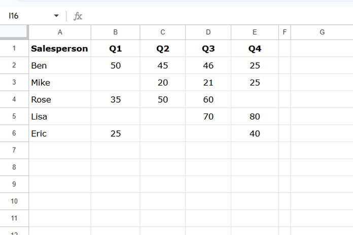
I want to use VLOOKUP to find Mike’s sales in Q1. The index column will be 2 in the VLOOKUP, and the formula would be as follows:

=VLOOKUP(G2, A2:E, 2, FALSE)

This formula will return a blank because the corresponding cell is empty. Therefore, you need the result from Q2. To get that, you would need to specify index number 3.

You can automate this process to dynamically adjust or move the index column in VLOOKUP in Google Sheets.

Formula Example of Moving the Index Column If Blank in VLOOKUP

In the above example, the data is in the range A1:E, and the lookup range is A2:E, excluding the header row.

Specify the salesperson’s name (the search key) in cell G2.

Then, enter the following formula in cell H2:

=IFERROR(
   INDEX(
      TOROW(
         VLOOKUP(G2, A2:E, SEQUENCE(COLUMNS(A2:E)+1-2, 1, 2), FALSE), 3
       ), 0, 1
   )
)

Where:

• Search key: G2
• Range: A2:E
• Index: 2

Note: You can simplify this formula using the LET function, and I will share that after the formula explanation.

When you use this formula for a different range, you only need to modify these arguments. I’ve highlighted them in the formula for your convenience.

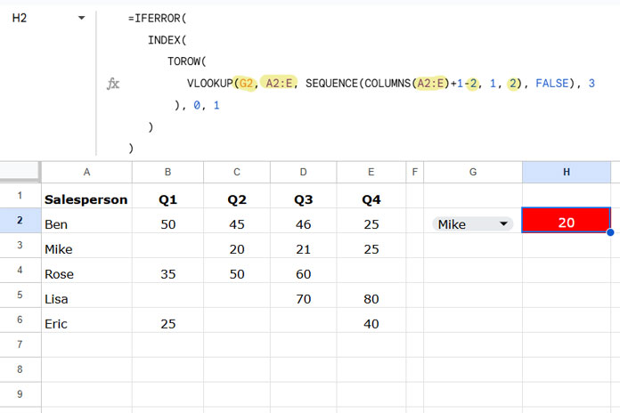
Even though the index is set to column 2, if VLOOKUP returns an empty value, it will fetch the value from the next non-blank cell in that row.

Let’s break down this formula to understand how we dynamically move the index column if it’s blank in the VLOOKUP formula in Google Sheets.

Formula Breakdown

The formula consists of three parts: the VLOOKUP part, the TOROW part, and the INDEX part. These work together to dynamically adjust, or we can say, move the index column if it is blank in VLOOKUP. Let’s break down each part in detail.

VLOOKUP Part:

VLOOKUP(G2, A2:E, SEQUENCE(COLUMNS(A2:E)+1-2, 1, 2), FALSE)

This follows the syntax:

VLOOKUP(search_key, range, index, [is_sorted])

Where:

• search_key: G2
• range: A2:E
• index: SEQUENCE(COLUMNS(A2:E)+1-2, 1, 2) – This generates a sequence of numbers corresponding to the columns in the range, starting from the specified index column. For example, if the index column is 2 and the range contains 5 columns, the formula will return the sequence numbers 2, 3, 4, and 5.
• is_sorted: FALSE

This VLOOKUP formula searches for the value in cell G2 in the first column of the range and returns the corresponding values from the columns specified by the index (in this case, columns 2 to 5).

When testing this formula standalone, you would need to wrap it with ARRAYFORMULA since the VLOOKUP index contains multiple columns. However, in our formula, we omit ARRAYFORMULA because the INDEX function works as an array formula.

TOROW Part:

TOROW(..., 3)

The purpose of the TOROW function is to remove any empty cells or errors in the result, if they exist, from the VLOOKUP.

INDEX Part:

INDEX(..., 0, 1)

The INDEX function extracts the first value from the row returned by the TOROW function.

This is how we dynamically move the index column if it’s blank in the VLOOKUP function in Google Sheets. Now, let’s simplify the formula using the LET function to make it easier to specify the arguments.

Simplified Formula for Moving Index Column If Blank in VLOOKUP

You can simplify the above formula using the LET function. With this function, we assign names to the search key, range, and index column, making it easier to specify them.

Here you go!

=LET(
   search_key, G2, range, A2:E, col_index, 2, 
   IFERROR(
      INDEX(
         TOROW(
            VLOOKUP(search_key, range, SEQUENCE(COLUMNS(range)+1-col_index, 1, col_index), FALSE), 3
         ), 0, 1
      )
   )
)

In this formula, you should specify:

• search_key: G2
• range: A2:E
• col_index: 2 (This represents the index; I used the name “col_index” to avoid conflicting with the INDEX function.)

That’s all about moving the index column if blank in VLOOKUP.

Sample Sheet

Resources

• Using VLOOKUP to Find the Nth Occurrence in Google Sheets
• Dynamic Index Column in VLOOKUP in Google Sheets
• Dynamic Column in Vlookup Importrange Formula in Google Sheets
• How to Get Dynamic Search Column in VLOOKUP in Google Sheets
• VLOOKUP: Skip Blank Cells and Continue Search – Google Sheets
• VLOOKUP to Get the Last Non-blank Value in a Row in Google Sheets