The ROWS function is a lookup function that returns the number of rows in a specified array or range in Google Sheets.
The output of the ROWS function has various potential uses in functions like HLOOKUP, SEQUENCE, INDIRECT, INDEX, etc.
Now, let’s explore the syntax of this function, basic use cases, and real-life applications. Here you go!
The Syntax and Arguments of the ROWS Function
Syntax:
ROWS(range)Arguments:
range: The range reference. It can be a physical range such as A1:A, A1:A100, B5:C10, A:Z, etc., or the output of any array formulas such as FILTER, UNIQUE, QUERY.
Basic Examples
To determine the number of rows in your entire sheet, you can specify any column in your sheet with an open range. Here is an example:
=ROWS(A:A)When you add or delete rows, this number will adjust accordingly.
Assuming you have some data in the range B2:D10. To find the number of rows in this range, use the following formula:
=ROWS(B2:D10)How do we use the ROWS function to find the number of rows in an array formula result?
Assume you have used the following FILTER formula to filter column A where column B=”Apple”:
=FILTER(A1:A,B1:B="Apple")To return the total number of rows in the result, simply wrap it with the ROWS function as follows:
=ROWS(FILTER(A1:A,B1:B="Apple"))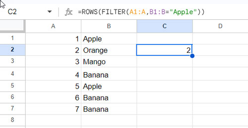
Let’s explore some real-world examples of the ROWS function in Google Sheets.
ROWS Function with the INDEX Function in Google Sheets
Assuming the last row in your table in the range A2:D7 contains totals and you are using the following INDEX formula to return the total:
=INDEX(A2:D7, 6, 4)Syntax of the INDEX Function:
INDEX(reference, [row], [column])Where:
A2:D7: This is the specified range where the data is located.6: This represents the row number. In this case, it’s the 6th row within the specified range.4: This represents the column number. In this case, it’s the 4th column within the specified range.
So, the formula is asking for the value in the cell that is in the 6th row and 4th column within the range A2:D7. Essentially, the total value in cell D7.
But what happens when you insert one row within the range?
The range within the formula will adjust and become A2:D8, yet the formula will return the value for cell D7.
You can solve this problem using the ROWS function.
Replace 6, which is the row number to offset, with the ROWS function, and here is that INDEX formula in cell B1:
=INDEX(A2:D7, ROWS(A2:D7), 4)
ROWS Function with the SEQUENCE Function in Google Sheets
With the SEQUENCE function, we can generate a grid of sequential numbers. Let’s explore how we can use it in combination with the ROWS function in Google Sheets.
Assume you want sequential numbers in a column starting from the current row, which is A5, to the end of the sheet. The following ROWS and SEQUENCE combo in cell A5 will return the numbers.
=SEQUENCE(ROWS(A5:A))Here is a scenario where you can see the full potential of the ROWS function and SEQUENCE function combo.
In the following example, we have names in column A and ages in column B:
=FILTER(A2:B, B2:B>9) // returns the names and ages for ages greater than 9How do we add a sequential number column to this result? Here it is:
=HSTACK(SEQUENCE(ROWS(FILTER(A2:B, B2:B>9))), FILTER(A2:B, B2:B>9))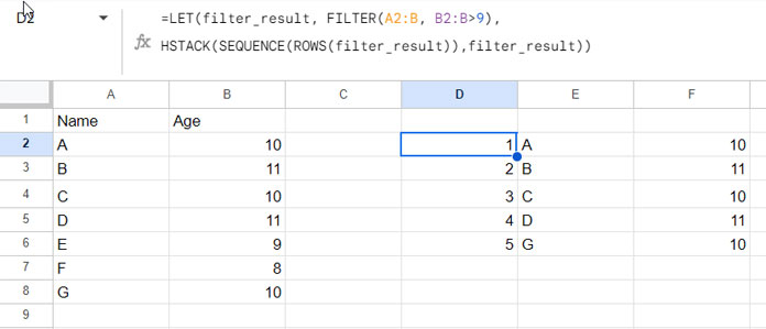
The SEQUENCE(ROWS(FILTER(A2:B, B2:B>9))) returns the sequential numbers, and the HSTACK function appends this with the filtered result.
We can avoid the repetition of calculation, which is the filter, by using the LET function as follows:
=LET(filter_result, FILTER(A2:B, B2:B>9), HSTACK(SEQUENCE(ROWS(filter_result)),filter_result))ROWS Function with the INDIRECT Function in Google Sheets
With the help of the ROWS function, we can dynamically define ranges in the INDIRECT function.
For example, if cell B2 contains a sheet name, the following formula will return the data from the range A2:Z in that sheet:
=INDIRECT(B2&"!A2:Z")Since the range is a string, it won’t dynamically adjust when you insert more columns in the referred sheet.
To address this issue in INDIRECT, you can use the ROWS function as follows:
=INDIRECT(B2&"!A2:"&ROWS(INDIRECT(B2&"!A1:A")))This formula works as follows:
B2&"!A2:": This part concatenates the content of cell B2 with the string"!A2:". If B2 contains, for example,Sheet1, then this part becomes"Sheet1!A2:".ROWS(INDIRECT(B2&"!A1:A")): The ROWS function returns the total number of rows in the INDIRECT range, i.e.,Sheet1!A1:A, if B2 contains the stringSheet1.- The above two parts combined to form a variable range within INDIRECT. If Sheet1 contains 1000 rows, the range within INDIRECT will be Sheet1!A2:A1000, an open range.
This formula allows you to reference a variable range in another sheet based on the sheet name in cell B2.
ROWS Function with the HLOOKUP Function in Google Sheets
The ROWS function is primarily useful in two ways within an HLOOKUP formula. In both cases, we will use it in the index part of the formula.
- To return the result from the last row of the matching column.
- To return results from all the rows in the matching column.
In the following sample data, I want to match the criterion “East” in row #1 in the range A1:E4 and return the value from the last row.
Here is the HLOOKUP and ROWS combination:
=HLOOKUP("South", A1:E4, ROWS(A1:E4), 0)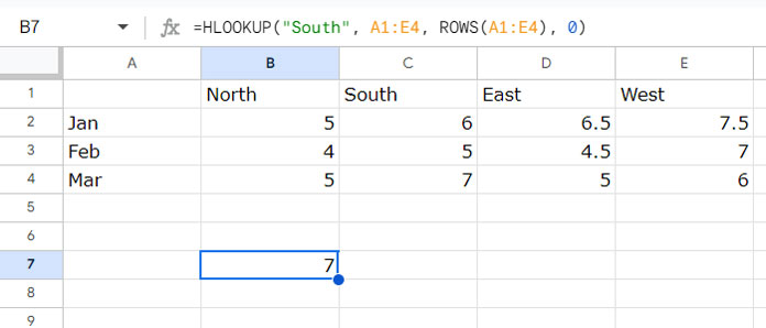
Syntax of the HLOOKUP Function:
HLOOKUP(search_key, range, index, [is_sorted])Where:
"South"is the search_key.A1:E4is the range.ROWS(A1:E4)is the index, representing the row number of the resulting column.0in is_sorted means the range is not sorted.
How do we return all the rows from the resulting column?
Just wrap the ROWS with SEQUENCE and enter it as an array formula as follows:
=ArrayFormula(HLOOKUP("South", A1:E4, SEQUENCE(ROWS(A1:E4)), 0))Related: How to Return an Entire Column in Hlookup in Google Sheets


