ISBLANK and COUNTBLANK are two functions that handle blank cells in Google Sheets. The former is an information function, while the latter is a mathematical function.
While the ISBLANK function checks a cell and returns TRUE if the cell is empty and FALSE otherwise, COUNTBLANK returns the count of blank cells in a range.
As this isn’t a comparison between ISBLANK and COUNTBLANK, let’s move on to discussing the usage of the ISBLANK function in Google Sheets.
Syntax:
ISBLANK(value)Where value is the value to check.
Examples
Assume cell A1 contains a value. The following formula will return FALSE:
=ISBLANK(A1)If you delete the value in cell A1, the formula will return TRUE.
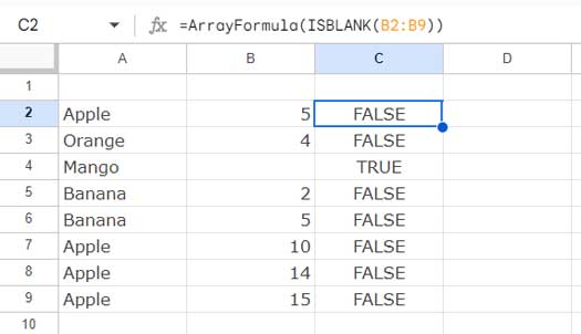
The ISBLANK function in Google Sheets can check blank cells in a range and return TRUE or FALSE values corresponding to the values in the range. Here is one such example:
How can I check if a pair of cells is not empty?
Suppose you want to verify that cells A1 and B1 are not empty and perform a task if both cells contain values. You can use either of these formulas:
=IF((ISBLANK(A1)+ISBLANK(B1)),, "do this task")
=IF(OR(ISBLANK(A1), ISBLANK(B1)),, "do this task")
Why Does the ISBLANK Function Return FALSE Even Though the Reference Cell is Empty?
Many of you may have noticed that ISBLANK returns FALSE even when the cell appears to be empty.
This discrepancy may be due to empty strings or hidden characters in the referenced cell. This often occurs when importing data into your sheet or when your formula returns empty strings. Here is an example of the latter scenario where we use an IF logical test.
The following formula in cell B1 returns an empty string (“”) if A1 contains “Verified”; otherwise, it returns “Please verify”.
=IF(A1="Verified", "", "Please verify")If cell A1 currently contains “Verified” and you check cell B1 using the ISBLANK function, it will return FALSE.
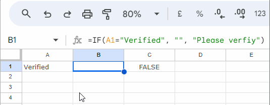
This explains why ISBLANK returns FALSE even though the source cell appears to be empty.
The correct way to use the IF logical test to return a blank cell is as follows:
=IF(A1="Verified", , "Please verify")ISBLANK Function in Data Validation
Data validation aids in maintaining data consistency. Here are two examples demonstrating how to utilize the ISBLANK function in data validation in Google Sheets:
Example 1: Allow entering values in a column if rows in another column have values.
You can implement the following rule to only allow entering values in column B if column A has values.
=ISBLANK(A1)=FALSETo apply this rule:
- Click Data > Data validation.
- Then click Add rule in the “Data validation rules” sidebar panel.
- Under “Apply to range,” enter the range to validate starting from cell B1. It can be just B1, or B1:B100 (from B1 up to the row you want).
- Under “Criteria,” select “Custom formula is”.
- Copy-paste the above formula into the given field.
- Check “Reject input” under “Advanced Options”.
- Click Done.
Example 2: Allow entering values in every other row of a column that corresponds to another column.
This is a slightly more advanced data validation rule.
=AND(ISODD(ROW(A1)), ISBLANK(A1)=FALSE)By replacing the previous rule with this one, it will permit you to enter values in B1, B3, B5, etc., provided A1, A3, A5, etc., have values.
ISBLANK Function in Conditional Formatting
Similarly to data validation, you can utilize the ISBLANK function in conditional formatting. Here is how to highlight all blank cells in a range.
Before writing the formula, you should decide the area to highlight. It can be a single cell or a range of cells. Whichever the case, the formula should reference the very first cell in the range.
Steps:
- Click Format > Conditional Formatting.
- Under “Apply to Range,” enter A1 or A1:C20 (the cell or cell range that you want to highlight).
- Under “Format Rules,” select “Custom formula is”.
- Enter
=ISBLANK(A1)in the provided field. - Select a formatting style and click Done.
Resources
Here are some additional resources related to managing blank cells in Sheets.
- How to Fill Zero in Blank Cells in Google Sheets
- Replace Blank Cells with 0 in Query Pivot in Google Sheets
- Array Formula to Fill Blank Cells With the Values from Cell Above
- How to Get Date Picker in Blank Cell in Google Sheets
- How to Highlight Blank Cells Using Value from Cell Above in Google Sheets
- How to Sort Rows to Bring the Blank Cells on Top in Google Sheets
- Two Ways to Specify Blank Cells in Google Sheets Formulas
- Count Blank Cells Row by Row in Google Sheets (COUNTBLANK Each Row)


I have 3 cells with costs.
1 cell has the original cost, and the other 2 “could” have discount costs ($ and %) OR will be BLANK if not used.
If there is no discount on the original cost, I want the original cost to be displayed in the totals cell.
What would the formula be?
D3 and D4 are the outcomes for each discount ($ and %), whereas B3 is the original cost.
Thank you for your help.
Hi, Paul Jamieson,
This may help.
=if(sumproduct(isblank(D3:D4))=2,B3,"")How do you use it on multiple cells at once?
For example, if any cells of A1, A2, and A3 are blank, then return TRUE, else FALSE.
How can you do that?
Hi, Michael K,
For that, we can use COUNTIF with ISBLANK.
E.g.:
=ArrayFormula(countif(isblank(A1:A3),TRUE))>0If my findings are correct, conditional formatting in a cell causes ISBLANK() to return FALSE.
For example, I use conditional formatting to gray out a cell that is empty. In the case of an empty cell,
LEN()returns zero andISBLANK()returns FALSE.Hi, Philip Milazzo,
It’s strange!
Can you please replicate the error for me in an example Sheet?
Best,