How to Sort Rows to Bring Blank Cells to the Top in Google Sheets

There are three methods you can use to sort rows and bring blank cells to the top in Google Sheets: the FILTER command, the QUERY function, and the SORT function with a helper column.

As a side note, there may be other methods, but I will focus on these three in this tutorial.

In this Google Sheets tutorial, you’ll learn how to use these three methods to sort rows to bring blank cells to the top in a column.

Sample Data

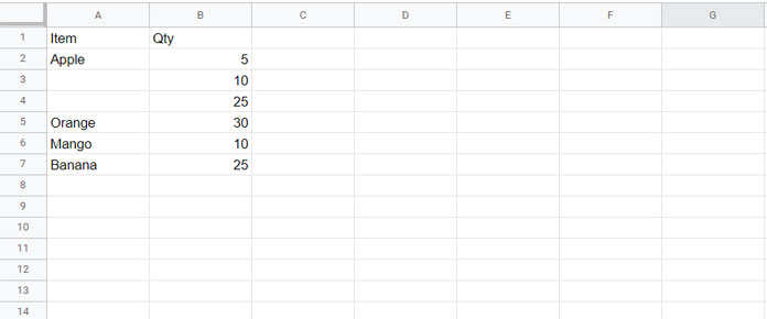
To illustrate the methods, let’s use a simple dataset with two columns and a few rows.

Sort Rows to Bring Blank Cells to the Top Using the FILTER Command

Google Sheets’ FILTER command (Data > Create a filter) provides sorting options that we can use for our purpose.

Steps:

Select the dataset (A1:B7), go to the menu Data, and click Create a filter.
Filter column A to bring blank cells to the top:
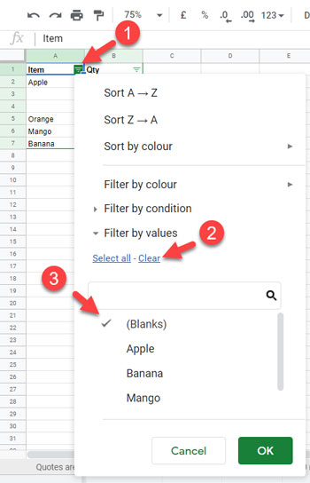
- Click the drop-down in cell A1.
- Click Clear.
- Select (Blanks).
- Click OK to isolate the blank cells.
Highlight the blank cells (A2:A3) by filling them with a color (e.g., Yellow).
Click the drop-down again, select Select all, and click OK.
Click the drop-down a third time and go to Sort by color > Fill color > Yellow.

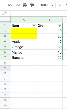
Move Blank Cells to the Top Using the FILTER Command

This method effectively sorts rows and brings blank cells to the top in Google Sheets. However, since sorting is applied based on fill color, only the blank cells will move to the top, while the other values will remain in their original order.

Sort Rows to Bring Blank Cells to the Top Using a QUERY Formula

A formula-based approach using the QUERY function allows you to populate the data in a new range with the desired sort order.

In Google Sheets, QUERY includes several clauses, and one of them is ORDER BY. We will use this along with the SELECT clause.

Formula:

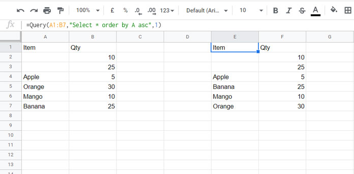
Enter the following formula in cell E1:

=QUERY(A1:B7, "SELECT * ORDER BY A ASC", 1)

This formula sorts the dataset while ordering blank cells first in column A.

Sort Rows to Bring Blank Cells to the Top Using QUERY

If you use this formula in a new sheet, include the sheet name with the range. For example:

=QUERY('Sheet1'!A1:B7, "SELECT * ORDER BY A ASC", 1)

Replace ‘Sheet1’ with the actual sheet name, ensuring it is enclosed in single quotes.

Why Not Use SORT or SORTN?

You might wonder why we don’t use SORT or SORTN to sort rows and bring blank cells to the top.

The SORT and SORTN functions place blank cells at the bottom in both ascending and descending order, whereas the QUERY function places blank cells on top in ascending order and at the bottom in descending order.

That said, if you’re unfamiliar with QUERY, you can still use SORT, but you’ll need a helper column.

SORT + Helper Column Approach

This method uses a helper column to sort rows and bring blank cells to the top.

Steps:

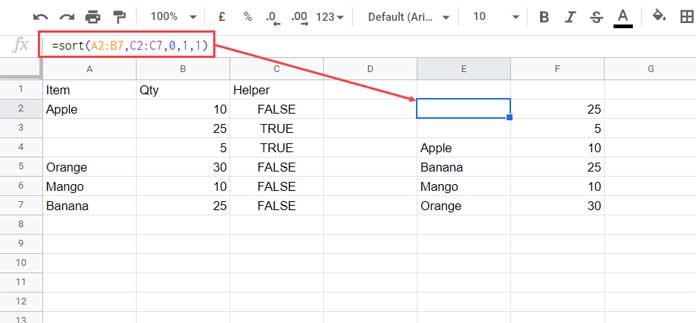
Insert the following formula in cell C1 (ensure column C is empty before doing this):
={"Helper"; ArrayFormula(A2:A7="")}
This formula marks blank rows with TRUE and non-blank rows with FALSE.
Use the following SORT formula in cell E2 to order blank cells first:
=SORT(A2:B7, C2:C7, FALSE, 1, TRUE)

This formula sorts column C in descending order (TRUE values first) while sorting column A in ascending order.

Sort Rows to Bring Blank Cells to the Top Using SORT

Conclusion

These are the three methods to sort rows to bring blank cells to the top in Google Sheets:

FILTER menu (manual approach)
QUERY formula (dynamic approach)
SORT with a helper column (alternative formula approach)

Each method has its use case, so choose the one that best fits your needs.

Thanks for reading! Enjoy working with Google Sheets.