We can use a combination formula rather than the SORT command in Google Sheets to sort data by custom order. In Excel, we can use either a formula or the SORT command, as explained in this Excel Guide: Custom Sort in Excel (Using Command and Formula).

The SORT function in Google Sheets allows you to sort your data in ascending or descending order. You can specify the sort by column (containing the values by which to sort) as either a column index or a range reference.

If the sort by column is outside the sort range, it’s not possible to specify the column index. In such cases, we will specify the range reference. We can leverage this peculiarity of the function to sort data by custom order in Google Sheets.

Syntax:

SORT(range, sort_column, is_ascending, [sort_column2, is_ascending2, …])

Arguments:

• range: The source data range.
• sort_column: The column index number or range reference indicating the column by which to sort. For example, you can use =SORT(A1:C10, 3, TRUE) or =SORT(A1:C10, C1:C10, TRUE) to sort the data range A1:C10 by the third column in ascending order. A range specified as a sort_column must be a single column with the same number of rows as the range.
• is_ascending: Indicating the sort order – TRUE for ascending or FALSE for descending.
• sort_column2, is_ascending2 …: [OPTIONAL] Additional columns and sort order.

As a side note, custom sorting is useful for sorting data by the status of tasks (pending, completed, in progress), types of cheques (PDC or CDC), hierarchy in an organization, and so on.

To sort by custom order, in addition to the SORT function, we may need to use one of the functions MATCH, XMATCH, or SWITCH.

Sorting Data by Custom Order in Google Sheets

Here is an example of sorting data by custom order in Google Sheets where A2:C8 contains customer names, cheque amounts, and modes of payment in columns A, B, and C respectively.

The modes of payment are “Pending,” “CDC” (current-dated cheque), and “PDC” (post-dated cheque). I want to sort the data in A2:C8 based on the values in C2:C8 in the custom order: “Pending,” “CDC,” and “PDC.”

Custom Sort Formula that Uses SORT and MATCH:

=SORT(A2:C10, MATCH(C2:C10, VSTACK("Pending", "CDC", "PDC"), FALSE), TRUE)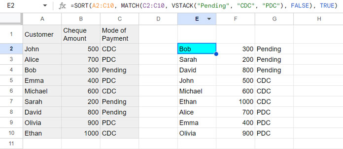

If you prefer to use XMATCH:

=SORT(A2:C10, XMATCH(C2:C10, VSTACK("Pending", "CDC", "PDC")), TRUE)

If you prefer to use SWITCH:

=SORT(A2:C10, SWITCH(C2:C10, "Pending", 1, "CDC", 2, "PDC", 3), TRUE)

Formula Explanation

In the above custom sort formulas:

• range: A2:C10
• sort_column: MATCH(C2:C10, VSTACK("Pending", "CDC", "PDC"), FALSE) or XMATCH(C2:C10, VSTACK("Pending", "CDC", "PDC")) or SWITCH(C2:C10, "Pending", 1, "CDC", 2, "PDC", 3)
• is_ascending: TRUE

So, the key to understanding the formula that sorts data by custom order in Google Sheets is the MATCH, XMATCH, or SWITCH formulas.

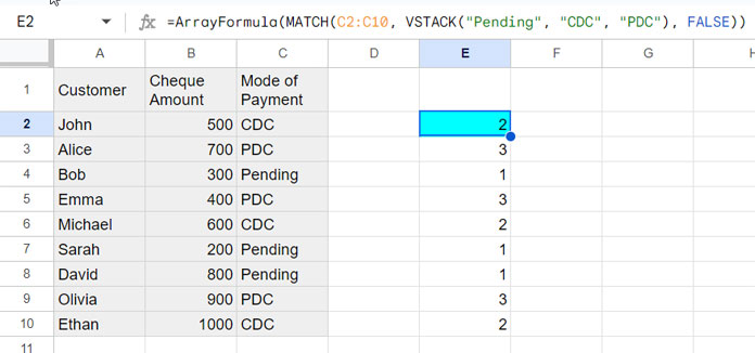
MATCH:

MATCH(C2:C10, VSTACK("Pending", "CDC", "PDC"), FALSE)

Syntax:

MATCH(search_key, range, [search_type])

The formula matches values in cell range C2:C10 (search_key) within a column that contains “Pending,” “CDC,” and “PDC” returned by VSTACK (range) and returns their relative positions.

The FALSE in MATCH represents an exact match of the search_key.

In short, it will assign the number 1 to “Pending,” 2 to “CDC,” and 3 to “PDC” for the values in the third column of the sort range.

When using XMATCH, you can omit the FALSE (which is equivalent to 0), as the default value is 0 (it won’t cause any issues if you keep FALSE).

Syntax:

XMATCH(search_key, lookup_range, [match_mode], [search_mode])

When using the SWITCH function, it tests cases in the expression and assigns the corresponding values.

SWITCH(C2:C10, "Pending", 1, "CDC", 2, "PDC", 3)

Syntax:

SWITCH(expression, case1, value1, [case2_or_default, …], [value2, …])

Sort By Custom Order and Assigning Header Row

As you can see, our data is in A1:C10, where A1:C1 contains the field labels. We omitted the header row when sorting the range as it might cause issues.

The functions that can recognize the field labels in Google Sheets are database functions and QUERY. The SORT function cannot recognize field labels.

So, to sort by custom order and assign the header row, use the VSTACK function as per the below generic formula.

Generic Formula: VSTACK(header_row, custom_sort_formula)

So, the formula will be:

=VSTACK(A1:C1, SORT(A2:C10, MATCH(C2:C10, VSTACK("Pending", "CDC", "PDC"), FALSE), TRUE))

Resources

In addition to the SORT function, we can also utilize the QUERY function to sort a range by custom order. Please check out the resources below:

1. Custom Sort Order in Google Sheets Query [Workaround]
2. How to Sort Pivot Table Columns in the Custom Order in Google Sheets
3. How to Custom Sort By Partial Match in Google Sheets