Have you ever needed to sort a list based on specific words contained within a text? Google Sheets doesn’t have a built-in function for this, but with a smart formula, you can achieve it effortlessly.
For example, imagine you have a list of T-shirts with different sizes (e.g., Classic Fit T-Shirt – XL, Cotton Crew Neck Tee – M, V-Neck Slim Fit Shirt – S), and you want to sort them from the smallest to the largest size based on a predefined order.
You can accomplish this using a combination of REGEXEXTRACT, XMATCH, and SORT functions.
Here’s the generic formula:
=SORT(range, IFNA(XMATCH(REGEXEXTRACT(range, "\b("&TEXTJOIN("|", TRUE, list)&")\b"), list)), TRUE)Where:
range– The dataset that you want to custom sort by partial match.list– A unique list defining the desired order for sorting (e.g., S, M, L, XL, 2XL, 3XL).
How to Custom Sort by Partial Match in Google Sheets (With Example)
Sample Data
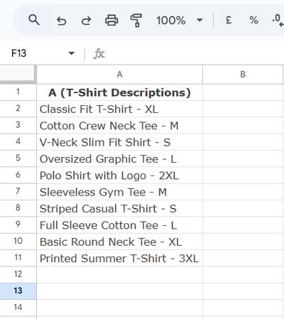
You have a list in column A (A2:A) with different T-shirt sizes mixed in text, like:
Now, in column C, you have the sorted unique sizes:
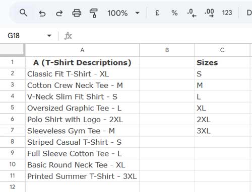
How do you sort column A by matching the sizes in column C from smallest to largest?
Formula to Custom Sort Data by Partial Match in Google Sheets
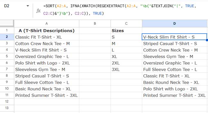
Use the following formula in cell D2 to sort the data:
=SORT(A2:A, IFNA(XMATCH(REGEXEXTRACT(A2:A, "\b("&TEXTJOIN("|", TRUE, C2:C)&")\b"), C2:C)), TRUE)This formula sorts the T-shirts in A2:A by partially matching the sizes in C2:C. Since the sizes are arranged from smallest to largest in column C, the output in column D will follow the same order.
Sorting in Descending Order
If you want to sort in descending order, replace TRUE with FALSE:
=SORT(A2:A, IFNA(XMATCH(REGEXEXTRACT(A2:A, "\b("&TEXTJOIN("|", TRUE, C2:C)&")\b"), C2:C)), FALSE)This will sort the T-shirts from largest to smallest.
How the Custom Sort by Partial Match Formula Works – Explained
This formula consists of four key parts:
1. TEXTJOIN – Creating the Search Pattern
TEXTJOIN("|", TRUE, C2:C)This joins the sorted size list (C2:C) into a single pattern separated by a pipe (|), which acts as an OR condition in regex. It also ignores empty cells.
Example output:
S|M|L|XL|2XL|3XLTo avoid incorrect matches, we wrap it with word boundaries (\b):
"\b("&TEXTJOIN("|", TRUE, C2:C)&")\b"This ensures only whole words match, preventing issues like “T-Shirt XL” accidentally matching “L” inside “XL.”
2. REGEXEXTRACT – Extracting the Matching Size
REGEXEXTRACT(A2:A, "\b("&TEXTJOIN("|", TRUE, C2:C)&")\b")This extracts the size from each T-shirt name in A2:A.
Example output:
| XL |
| M |
| S |
| L |
| 2XL |
| M |
| S |
| L |
| XL |
| 3XL |
3. XMATCH – Getting the Position of Each Size
IFNA(XMATCH(REGEXEXTRACT(A2:A, "\b("&TEXTJOIN("|", TRUE, C2:C)&")\b"), C2:C))- XMATCH finds the extracted size in the sorted list (C2:C) and returns its position in the list.
- IFNA prevents errors if there’s no match.
Example output:
| Extracted Size | XMATCH Result |
| XL | 4 |
| M | 2 |
| S | 1 |
| L | 3 |
| 2XL | 5 |
| M | 2 |
| S | 1 |
| L | 3 |
| XL | 4 |
| 3XL | 6 |
4. SORT – Arranging Data by Extracted Positions
=SORT(A2:A, IFNA(XMATCH(REGEXEXTRACT(A2:A, "\b("&TEXTJOIN("|", TRUE, D2:D)&")\b"), D2:D)), TRUE)- SORT arranges T-shirts based on the size order from C2:C.
- The final result is a sorted list of T-shirts from smallest to largest size.
Final Thoughts
Sorting data by a partial match in Google Sheets is not possible with built-in sorting, but this method provides a powerful custom sort by partial match approach. By using REGEXEXTRACT, XMATCH, and SORT, you can dynamically arrange lists based on specific text patterns.


