Array formulas often break or mess up if they are located within the range being sorted. So, can we prevent array formulas from breaking or messing up during sorting in Google Sheets?
In most cases, we can. The simple solution is to move the array formula one row above the sort range. I’ll explain how to adjust the formula for this. However, this approach may not work in all scenarios.
Let’s explore an example of an array formula that messes up and breaks in a particular case when sorting in Google Sheets.
Understanding the Problem
In the example below, there’s an array formula in cell C2 that assigns grades to students based on their scores.
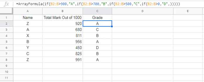
Formula:
=ArrayFormula(IF(B2:B>900, "A", IF(B2:B>700, "B", IF(B2:B>500, "C", IF(B2:B>0, "D",)))))It uses a nested IF structure to work as follows:
- If the “Total Mark Out of 1000” is greater than
900, the formula assigns a grade of “A”. - If the marks are greater than
700, it assigns “B”. - If the marks are greater than
500, it assigns “C”. - Otherwise, it assigns “D”.
This grading is done using a single array formula in column C.
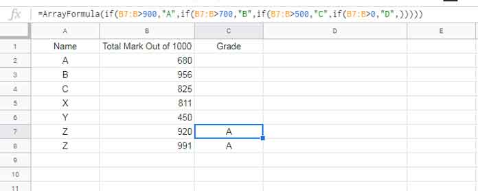
Now, let’s say I want to sort the student names alphabetically. To do this, I select the range A2:C8 and sort the data using Data > Sort range > Sort range by column A (A to Z).
After sorting, check column C. You’ll see that the sorting has messed up the array formula because the row containing the formula moved during the sort.
Solutions to Array Formula Messing Up in Sorting
To prevent array formulas from messing up during sorting in Google Sheets, you can use a simple trick: enter the array formula outside the sort range. For instance, instead of placing the array formula in cell C2, enter it in C1.
However, the formula will need slight modifications. Use the following syntax:
={"column name"; arrayformula}This format appends a column name to the array formula, ensuring it integrates smoothly with the header row. Let’s explore two approaches based on different sorting scenarios.
Option #1: Prevent Sorting from Messing Up the Array Formula
For the example above, here’s the modified array formula:
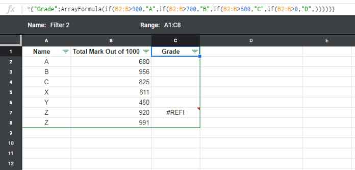
={"Grade"; ArrayFormula(IF(B2:B>900, "A", IF(B2:B>700, "B", IF(B2:B>500, "C", IF(B2:B>0, "D",)))))}Enter this formula in cell C1, not C2. Since row 1 isn’t part of the sort range, the formula remains unaffected during sorting.
This solution works well in most cases. You can sort the data using Data > Sort range or apply a filter and sort using Data > Create a Filter, then selecting A-Z or Z-A from the filter drop-down.
However, if you use Data > Create filter view, the sorting will break the formula. To prevent this, you need to modify the array formula itself. Let’s explore the fix below.
Option #2: Prevent Filter View Sorting from Breaking the Array Formula
Here’s a solution that works for both cases:
=ArrayFormula(IF(ROW(A:A)=1, "Grade", IF(B:B>900, "A", IF(B:B>700, "B", IF(B:B>500, "C", IF(B:B>0, "D",))))))How does this formula differ from the Option #1 formula?
This formula uses full column ranges, such as A:A and B:B, instead of partial ranges like A2:A or B2:B. Avoid using ranges like A1:A or B1:B, as they can still cause the formula to break during sorting.
- In the first row, the formula returns the header, controlled by the condition
IF(ROW(A:A)=1, "Grade", ...). - For all other rows, the formula performs the actual calculations.
By using this method, the array formula remains unaffected, regardless of whether sorting is performed via Data > Sort range, Data > Create a Filter, or Data > Filter view.
Conclusion
Array formulas can break when sorting data in Google Sheets, but with the right adjustments, you can prevent this. Moving the formula to the header row and modifying it to accommodate sorting ensures smooth operation.


Great explanation. Would option two work using Table ranges instead of the full column? Thanks!
Thank you for your question! Unfortunately, using table ranges wouldn’t work in this case, as table ranges don’t support formulas in the header row.
Hi Sir,
I am sending the link for the file.
[Spreadsheet ID]
Thanks,
Pradeep
Thanks for sharing your sheet. You can use my most recent formula. Just replace
DescwithAscin the QUERY.Hi,
Thanks a lot! In hindsight, I think I should have been able to figure it out, but as I mentioned before, I’ve never used GS before, so the syntax was a bit too much for me.
Thanks again!
Pradeep
Glad to be of help.
Hi Prashanth,
I am so happy to tell that your solution worked perfectly. I am sorry that I posted this on the wrong topic page because I thought it was more to with array sorting rather than the monthly output; as I was getting it anyways with my formula.
Thanks again!!
Hi Prashanth,
I am trying to adapt your array sort method for my query.
=ARRAYFORMULA(SORTN(TEXT(GOOGLEFINANCE(B2, "close", TODAY()-1000,TODAY(),1),{"yyyy mm ", "@"}), 9^9, 2, 1, 0))
I am using this formula to pull down the closing price of a stock. The output data is in this format:
Date Value
2023-08 100
2023-07 106
…and so on.
However, I want to present this output in reverse order. The oldest date should be first, and the most recent date should be last.
I appreciate your help in advance.
Hi Pradeep,
I believe you posted your question in the wrong topic.
The issue with your formula is that the text formatting is preventing you from sorting the data in the desired order.
I suggest you use the following formula, which is the correct way to achieve your desired result.
=LET(gf,QUERY(GOOGLEFINANCE(B2, "close", TODAY()-1000,TODAY(),1),"Select * Offset 1",0),SORTN(HSTACK(EOMONTH(INT(CHOOSECOLS(gf,1)),-1)+1,
CHOOSECOLS(gf,2)),9^9,2,1,1))
You can find this approach in my EOMONTH function under the subtitle “The Role of EOMONTH in QUERY.”
I wanted the last date of the month instead of the first date.
I am new to Google Sheets, and there is nothing like this in Microsoft Excel. I hope you will be so kind as to help me again.
Many thanks,
Pradeep
I understand. Here is the formula. It will return the actual month-end date in the GOOGLEFINANCE result with timestamp, instead of the month-end dates.
=LET(data,QUERY(GOOGLEFINANCE(B2, "close", TODAY()-1000,TODAY(),1),"Select * Order By Col1 Desc Offset 1",0),
SORTN(data,9^9,2,EOMONTH(CHOOSECOLS(data,1),-1)+1,1))
Dear Prashanth,
Sorry to bother you again. This formula is also giving the closing prices of the actual month-end date. But I need the closing price on the first day of the month.
Could you take a second look?
Thanks
Pradeep
Please create a sample sheet with sample data and hand-entered expected results. Copy the URL and share it in view mode below.
Hi Prashanth, great post!
Just have one question,
How would you include a SUM of all the values just below the header without:
– Messing up the SUM row order
– Getting a circular dependency
Hi, Damien Lemaitre,
I didn’t get “Messing up the SUM row order.”
Please clarify and also share an example.
This is a great option, I can’t seem to get the array to calculate the last row in the column.
=ArrayFormula(if(row(A:A)=1,"ID",IF(isblank(H:H),"",ifna(vlookup($G$2:$G,Codes!$I$2:$J,2,false))&" - "&
ifna(vlookup($D$2:$D,Codes!$C$2:$D,2,false))&
ifna(vlookup($E$2:$E,Codes!$E$2:$F,2,false))&
ifna(vlookup($F$2:$F,Codes!$A$2:$B,2,false))&$V$2:$V&
ifna(vlookup($C$2:$C,Codes!$G$2:$H,2,false))))
)
There is a value in H, the result for the last row is that it only puts in the ” – ” but nothing from the lookup values.
If I add another row at the bottom, it works fine with the previous last row.
I figured it out. I had the G2:G type reference instead of G:G.
Is there a way to prevent it from putting 0’s all the way to the end of the column? What did I miss?
here is my formula:
=ArrayFormula(if(row(A:A)=1,"Days Rest",IF(J:J<21,"0",if(J:J<36,"1",if(J:J<51,"2",if(J:J<65,"3",if(J:J<86,"4")))))))I also have this one in the next column, any idea how to make it a date format?
=ArrayFormula(IF(row(A:A)=1,"Eligible Date",(To_Date(C:C+K:K))))Fixed it adding the initial IF to check ISFBLANK.
=ArrayFormula(if(row(A:A)=1,"Days Rest",IF(isblank(J:J),"",IF(J:J<21,"0",
IF(J:J<36,"1",if(J:J<51,"2",
if(J:J<65,"3",if(J:J<86,"4"))))))))
Still working on the date column.
Hi Steven,
Maybe by including the DATEVALUE function and an IFERROR.
=ArrayFormula(IFERROR(IF(row(A:A)=1,"Eligible Date",if(datevalue(C:C),To_Date(C:C+K:K)))))Best,
Thanks, still just a number. 🙁
This seems to work:
Put the to_date at the beginning.
=ArrayFormula(to_date(IFERROR(IF(row(A:A)=1,"Eligible Date",if(Datevalue(C:C),(C:C+K:K))))))Thanks!
Hi, SKS,
I am glad that you find the tips useful.
Best,
Great post.
I had faced this problem many a time but was not able to find any solution.
This trick will be really helpful.