How to Skip a Total in the Query Total Row in Google Sheets

Sometimes, small tips can make a big difference in getting your formulas to work just right. One such trick is how to insert a blank cell between two totals in a Query total row in Google Sheets.

You may not always need it, but when you do, this simple workaround comes in handy.

This guide is part of the QUERY Pivot & Reporting in Google Sheets series and focuses on adding totals selectively to specific columns in QUERY pivot reports.

Table of Contents

Example of Skipping a Total in the Query Total Row

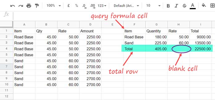
Here’s a sample sales dataset in A1:D.

Screenshot of sample sales data and the expected Query output showing a blank cell between two totals in the total row in Google Sheets

Since this tutorial includes step-by-step instructions (with the final formula coming in two main steps), you may want to recreate the same dataset in your sheet using the range A1:D.

In this example, I’ve summarized the sales data by grouping column A — which contains items like “Road Base” and “Sand.”

You’ll find the summary output in the range F1:I. (We’ll get to the formula in a moment.)

In the summary, we’re aggregating columns B, C, and D. Columns B (Qty) and D (Amount) are summed, while column C (Rate) is averaged using the QUERY function.

Now here’s the catch: we don’t want to show the total of the average column (Rate) in the total row. So the goal is to skip the total of column C and instead leave a blank cell in its place — like what you see in cell H4.

Let’s walk through how to do it.

Step 1: Query Summary (Grouping and Aggregation)

Let’s first write the QUERY formula for the grouped summary.

Query Summary Formula:

=QUERY(
  A1:D,
  "SELECT A, SUM(B), AVG(C), SUM(D) WHERE A IS NOT NULL GROUP BY A LABEL SUM(B) 'Quantity', AVG(C) 'Rate', SUM(D) 'Total'",
  1
)

Quick Breakdown:

Group by column A:
We’re grouping on column A using both SELECT A and GROUP BY A.
Aggregate the other columns:
- Column B → SUM(B)
- Column C → AVG(C)
- Column D → SUM(D)
WHERE clause:
The WHERE A IS NOT NULL clause avoids pulling in any blank rows from the dataset (especially if your range goes beyond the last data row).
LABEL clause:
This customizes the output column names for readability.

You can skip the LABEL part if you’re okay with default labels.

Step 2: Generate a Total Row and Skip One Total

Now let’s create a total row that leaves the average (column C) blank.

Start by modifying the previous formula. This time, remove column A and the GROUP BY clause entirely:

=QUERY(
  A1:D,
  "SELECT SUM(B), AVG(C), SUM(D) WHERE A IS NOT NULL LABEL SUM(B) 'Quantity', AVG(C) 'Rate', SUM(D) 'Total'",
  1
)

This gives us the total row.

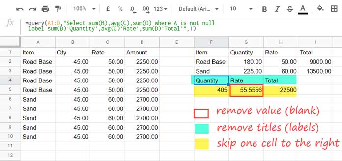
Query summary with total values shown for all aggregated columns including quantity, rate, and amount

Tip 1 – Insert a Blank Cell Between Two Totals

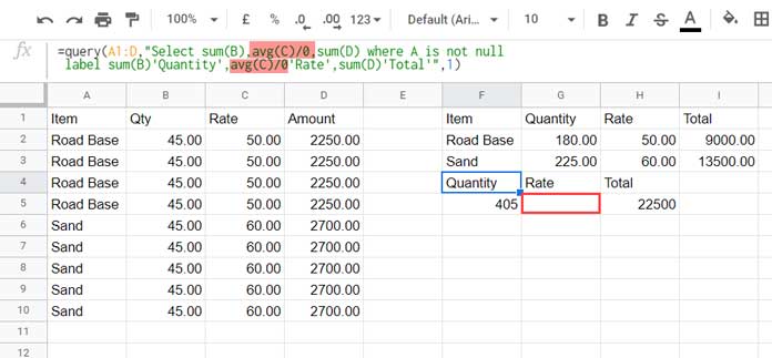
To skip the total for column C, we’ll force a blank by dividing the AVG(C) by zero. This results in a #DIV/0! error, which Google Sheets treats as a blank in the QUERY output.

Here’s the modified formula:

=QUERY(
  A1:D,
  "SELECT SUM(B), AVG(C)/0, SUM(D) WHERE A IS NOT NULL LABEL SUM(B) 'Quantity', AVG(C)/0 'Rate', SUM(D) 'Total'",
  1
)

Example of how to skip a total in the Query total row in Google Sheets using a blank cell in the rate column

Tip 2 – Remove Labels from the Total Row

To remove the header row from the total query, just wrap the formula with CHOOSEROWS(..., 2) to select the second row only (the total row).

=CHOOSEROWS(
  QUERY(
    A1:D,
    "SELECT SUM(B), AVG(C)/0, SUM(D) WHERE A IS NOT NULL LABEL SUM(B) 'Quantity', AVG(C)/0 'Rate', SUM(D) 'Total'",
    1
  ),
  2
)

Tip 3 – Add a Custom Label Like “TOTAL”

To add a label like “TOTAL” in the first column, use HSTACK to combine your total row with a static value:

=HSTACK(
  "TOTAL",
  CHOOSEROWS(
    QUERY(
      A1:D,
      "SELECT SUM(B), AVG(C)/0, SUM(D) WHERE A IS NOT NULL LABEL SUM(B) 'Quantity', AVG(C)/0 'Rate', SUM(D) 'Total'",
      1
    ),
    2
  )
)

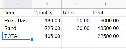
Total row in a Query output with column labels removed and a blank cell between two totals

Final Step – Combine Summary and Total Rows

Now let’s combine the summary table and the total row using VSTACK:

=VSTACK(
  QUERY(
    A1:D,
    "SELECT A, SUM(B), AVG(C), SUM(D) WHERE A IS NOT NULL GROUP BY A LABEL SUM(B) 'Quantity', AVG(C) 'Rate', SUM(D) 'Total'",
    1
  ),
  HSTACK(
    "TOTAL",
    CHOOSEROWS(
      QUERY(
        A1:D,
        "SELECT SUM(B), AVG(C)/0, SUM(D) WHERE A IS NOT NULL LABEL SUM(B) 'Quantity', AVG(C)/0 'Rate', SUM(D) 'Total'",
        1
      ),
      2
    )
  )
)

And that’s it! You now have a summary table with a custom total row — and a blank cell in place of a column you didn’t want totaled.

Wrap-Up

Using this trick, you can easily skip a total in the Query total row in Google Sheets, whether it’s an average column or something else you don’t want totaled. The divide-by-zero trick and HSTACK/VSTACK combo let you fully customize your Query output — without any manual editing.