Counting words and inserting corresponding blank rows may not be a common task in Google Sheets, but it can be highly useful in certain situations.
For instance, when preparing data for presentations or organizing entries for analysis, inserting blank rows provides clearer separation of data. This method allows you to insert a specific number of blank rows beneath each row based on the number of words in the cell.
This technique is particularly useful for:
- Commenting: When blank rows are inserted below a cell, they can be used to leave comments or annotations for each word in adjacent columns.
- Structured data manipulation: When working with large datasets, it helps create space to input additional information related to the initial data.
Note: You can’t enter values directly in cells that are part of an array formula output. If you need to edit or manually input values, first copy the result and paste it as values. To do this, right-click on the output, select “Copy” from the shortcut menu, then right-click again and choose “Paste Special” to paste as values.
Example Scenario
Suppose you have a dataset where each cell contains fruit names separated by commas or pipes. The goal is to count the number of fruits (or words) in each cell and insert an equivalent number of blank rows beneath the original data.
For example:
- If cell B2 contains “Apple, Banana, Mango,” three blank rows will be inserted beneath it.
- If cell B3 contains “Orange, Grape,” two blank rows will follow.
In this example, here’s a formula you can use in cell C2:
=ArrayFormula(
   LET(
      range, B2:B3,
      words, IF(range="",,LEN(range)-LEN(SUBSTITUTE(range,",", ""))+2),
      data, TOCOL(HSTACK(range, MAP(words, LAMBDA(val, IFNA(WRAPROWS(, val)," ")))), 2),
      FILTER(data, data<>"")
   )
)
Replace B2:B3 with the actual range where your data is located. If your data uses a different delimiter (e.g., pipe |), replace the comma in the SUBSTITUTE function accordingly.
Example of Counting Words and Inserting Blank Rows
Let’s say column A contains the following data, where the words are pipe-delimited:
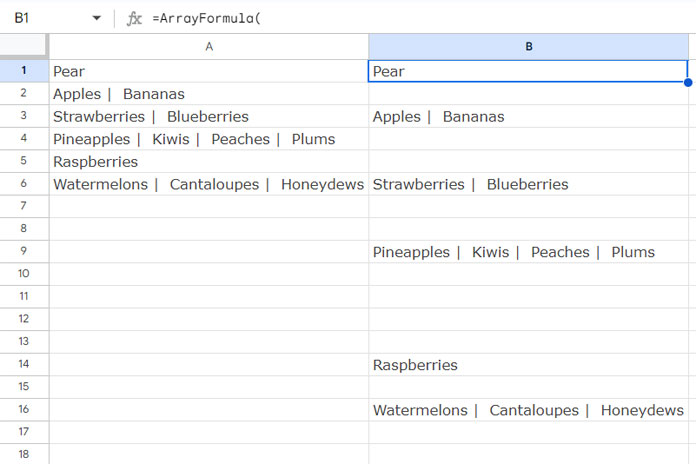
You can use the following formula in cell B1 to count the number of words in A1:A and insert the corresponding number of blank rows.
=ArrayFormula(
   LET(
      range, A1:A,
      words, IF(range="",,LEN(range)-LEN(SUBSTITUTE(range,"|", ""))+2),
      data, TOCOL(HSTACK(range, MAP(words, LAMBDA(val, IFNA(WRAPROWS(, val)," ")))), 2),
      FILTER(data, data<>"")
   )
)
Formula Breakdown
- LET Function: The LET function simplifies complex formulas by allowing you to define variable names for portions of the formula, making it easier to read and improving performance.
- range:
A1:A
This represents the data range where words are separated by a delimiter (e.g., pipes|). - words:
IF(range="",,LEN(range)-LEN(SUBSTITUTE(range,"|",""))+2)
This calculates the number of words in each cell by subtracting the length of the string after removing the delimiter and adding two. Normally, we would add one to account for the final word without a delimiter, but here we add two, which we will explain below.- Output Example:
{2; 3; 3; 5; 2; 4}
- Output Example:
- data:
TOCOL(HSTACK(range, MAP(words, LAMBDA(val, IFNA(WRAPROWS(, val)," ")))), 2)WRAPROWS(, val): Creates cells filled with#N/Abased on the word count (val) except for the first one, which is left blank. We will remove this empty cell and use the#N/Acells. This is why we added 2 to the word count instead of 1 in the earlier step.IFNA(WRAPROWS(, val)," "): Replaces#N/Awith a space (” “).MAP(words, LAMBDA(val, ...)): Applies this operation for each word count in the array.HSTACK(range, ...): Horizontally stacks the original range and the blank rows generated.TOCOL(..., 2): Converts the horizontally stacked data into a column, removing errors.
FILTER(data, data<>"")
TheFILTERfunction removes any remaining empty cells, ensuring only meaningful data and blank rows remain.
Additional Use Cases
Beyond data presentation and structure, here are some other potential uses for this approach:
- Align Data for Visual Comparison: Insert blank rows between data entries to create visual separation, making it easier to compare items from different categories without merging them into a single table.
- Add Space for Notes or Feedback: Use this method in collaborative environments to allow users to leave feedback, comments, or notes in rows next to each data entry, ensuring clarity and organization.
- Customizing Data Formatting for Export: When exporting data from Google Sheets for use in other platforms or reports, inserting blank rows may help improve the format or structure of the exported data.
Resources
- How to Insert Blank Rows Using a Formula in Google Sheets
- Automatically Insert Blank Rows Between Groups in Google Sheets
- Insert Blank Rows to Separate Week Starts/Ends in Google Sheets
- How to Insert Duplicate Rows in Google Sheets
- Insert Subtotal Rows in a Google Sheets Query Table
- Expand Dates and Assign Values in Google Sheets (Array Formula)
- Insert Blank Rows After Each Category Change in Excel
- EXPAND + Stacking: Expand an Array in Excel


I tried to leave a comment here yesterday, but it seems like I failed somehow…
So, what I was wondering was if you know if there is a way to instead turn this:
Student1, Student2, Student3 | Monday
Student4, Student 5 | Tuesday
Student6 | Wednesday
Student7, Student8 | Thursday
Student9 | Friday
Into this:
Student1 | Monday
Student2 | Monday
Student3 | Monday
Student4 | Tuesday
Student5 | Tuesday
Student6 | Wednesday
Student7 | Thursday
Student8 | Thursday
Student9 | Friday
It seems like it should be easy enough. But the deeper into it I get, the more impossible it seems. I’m having big trouble getting the different items from the comma-separated string into the new rows. And especially if I also want to copy some other value (like from the Allocation column) from the correct row.
Hi,
I have already a solution for the same. Here it is – Split to Column and Categorize.
I have one more solution using a different function (FLATTEN). I’ll post it soon and update you below.
Hello,
You can read this new tutorial.
Split Comma-Separated Values in a Multi-Column Table in Google Sheets.
Hi, Prashanth,
Can you please assist me with a similar problem. I would like to convert a 2 column array into multiple tables based on the data in the 2 columns. The array data is based on an import and changes each time new data is imported.
The formula must essentially count repeats in column A and insert that count +1 (to include a space between the tables) while also inserting the associated values from column B into the spaces between.
Please see the example spreadsheet here: … sheet’s URL removed by admin …
Hi, Jordan,
You have a category column (column A) and a value column (column B). To merge this into one column you can try the below formula.
=filter(flatten({if(COUNTIFS(A3:A,A3:A,ROW(A3:A),"<="&ROW(A3:A))=1,A3:A27,),B3:B}),flatten({if(COUNTIFS(A3:A,A3:A,ROW(A3:A),"<="&ROW(A3:A))=1,A3:A27,),B3:B})<>"")It won’t insert any blank rows in between. If you want a detailed explanation for this formula, please let me know. I’ll consider writing a tutorial then.
Thank you very much, Prashanth! Yes, can you please write a detailed explanation? Just so that I can refer back to it if I need to tweak the formula in the future
If I wanted to add a space in between, is it possible to use a helper column or adding column c with only spaces in each cell?
Hi, Jordan,
Here you go!
How to Merge Two Columns Into One Column in Google Sheets.
Regarding your query to add a space in between merged columns, please see the tab “TABLE 2 blank row” in the shared sheet at the end of the above post.
Legend! Thank you very much 🙂