Insert Blank Rows to Separate Week Starts/Ends in Google Sheets

Sometimes, we may want to insert blank rows to separate week starts or ends in Google Sheets. How do we do it?

Of course, inserting blank rows between each change in weeks in a date column can be useful for improving readability and making printed copies of reports look cleaner.

If you have a large dataset, manually doing this can be tedious. That’s why we’ve created formulas to automate the process for you.

Let’s approach this from two different perspectives:

Inserting blank rows at every week change row in existing data.
Generating a sequence of dates separated by every week change.

In this post, we will share two formulas that serve the above purposes, starting with the existing data.

The formulas have the following key features:

They are array formulas.
They do not use helper cells.
You can increase or decrease the number of blank rows to insert at every week change row.
You can use any day of the week as the separator.

How to Insert Blank Rows to Separate Week Starts or Ends in Google Sheets

Click the button below to copy my sample Sheet.

sample_111023

Now, let’s go to the examples.

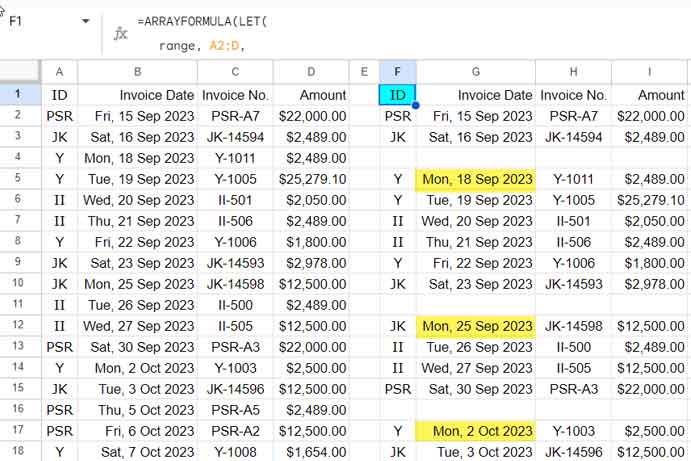
In the following example, I have an outstanding liability statement in Google Sheets that is sorted by invoice dates. I want to insert blank rows to separate every week’s start, which is Monday.

The statement contains four columns: ID, Invoice Date, Invoice Number, and Amount.

In the following screenshot, you can see the sample data in A1:D and the formula result in F1:I. The formula in F1 populates the entire result.

Image of a Google Sheets spreadsheet with blank rows inserted to separate week starts or ends.

Prerequisites

To use the formula, you need to know the following:

Data range: The range of cells that contains your data, excluding the header row.
Header row range: The range of cells that contains the header row.
Date column range: The range of cells that contains the date column.
Day of the week starts: The day of the week that you want to use as the separator. Use one of the numbers from 11 to 17, where 11 is Monday and 17 is Sunday.

Formula

The following formula in Google Sheets inserts blank rows to separate weeks that start on Monday. In other words, it inserts a blank row after every week that ends on Sunday.

=ARRAYFORMULA(LET(
   range, A2:D,
   header, A1:D1,
   dt, B2:B,
   at, 11,
   helper, WEEKNUM(DATEVALUE(dt),at),
   REDUCE(header,TOCOL(UNIQUE(helper),3),
   LAMBDA(a,v,IFERROR(VSTACK(a,FILTER(range,helper=v),))))
))

To insert a blank row to separate weeks that start on Sunday and end on Saturday, replace 11 in the formula with 17.

How to Insert Two Blank Rows Below Each Week Change

To insert two blank rows below each week change in a date column, add one more comma to the last part of the formula. For example:

=ARRAYFORMULA(LET(
   range, A2:D,
   header, A1:D1,
   dt, B2:B,
   at, 11,
   helper, WEEKNUM(DATEVALUE(dt),at),
   REDUCE(header,TOCOL(UNIQUE(helper),3),
   LAMBDA(a,v,IFERROR(VSTACK(a,FILTER(range,helper=v),,))))
))

The formulas above can be used to insert blank rows to separate week starts or ends in Google Sheets. The formulas are flexible and can be customized to meet your specific needs.

Formula Explanation

In short, the above formula is a combination of the functions WEEKNUM, UNIQUE, and REDUCE.

WEEKNUM: Returns the week number of a date, given the day of the week that the week starts on. In this case, the week starts on Monday.
UNIQUE: Returns a unique list of values from an array.
REDUCE: Reduces an array of values to a single value by applying a function to each element of the array and accumulating the results.

Let’s see how the formula inserts blank rows to separate week starts or ends.

Week Numbers

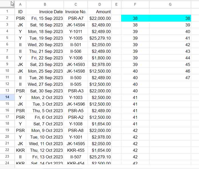
To test the formula, you can keep only the sample data in A1:D. Then, insert the following formula in cell F2 to return the week number of the dates in A2:A, with the week starting on Monday:

=ARRAYFORMULA(WEEKNUM(DATEVALUE(B2:B),11))

The DATEVALUE function ensures that the WEEKNUM function only returns the week number of non-blank cells. Usually, the WEEKNUM function returns a number even if the cell is blank, which can cause formula errors.

Unique Week Numbers

Next, insert the following UNIQUE formula in cell G2:

=TOCOL(UNIQUE(F2:F),3)

The TOCOL function ensures that the unique week numbers do not contain an error value.

Insert Blank Row Below Week Change Row: Explained with Helper Columns

Lambda Function

Finally, insert the following REDUCE formula in cell I2, which is the complex part to understand.

=REDUCE(A1:D1,G2:G11,LAMBDA(a,v,IFERROR(VSTACK(a,FILTER(A2:D,F2:F=v),))))

The REDUCE function works by applying a lambda function to each element of the array and accumulating the results.

The lambda function in this formula takes two arguments: a and v.

a is the accumulator, which is the result of applying the lambda function to all of the previous elements of the array.
v is the current element of the array.

Note: The array here is G2:G11, which contains the unique week numbers and the current element of the array is G2. The current value in the accumulator is A1:D1 (initial value in the accumulator).

The lambda function returns all of the rows in the data range (A2:D) that have the same week number (v) by matching v in F2:F.

FILTER(A2:D,F2:F=v)

The REDUCE function then applies the VSTACK function to the accumulator and the result of the lambda function, then a blank cell.

VSTACK(a,FILTER(A2:D,F2:F=v),)

This stacks the three arrays vertically, creating a new array that contains the initial value (header row) and all of the rows in the data range that have the same week number as the G2, then a row with error values because of the comma we placed in VSTACK.

The REDUCE function then continues to iterate over the array of unique week numbers (G2:G11), applying the lambda function and the VSTACK function to each element of the array.

The IFERROR removes the errors and returns blanks. The result is a single array that contains all of the rows in the data range, with blank rows inserted to separate week starts.

Generate a Sequence of Dates and Separate Week Starts or Ends with Blank Rows

Sometimes, we want to generate a sequence of dates and separate week starts or ends with one or more blank rows. In this case, we can use the formula above by replacing the data range with a SEQUENCE formula. We do not need to specify the date range because we have only one column.

For example, you want to generate a sequence of 100 dates in sequential order starting from the date specified in cell A1. The following formula will take care of that:

=ARRAYFORMULA(LET(
   range, SEQUENCE(100,1,A1),
   header, "text",
   at, 11,
   helper, WEEKNUM(range,at),
   REDUCE(header,TOCOL(UNIQUE(helper),3),
   LAMBDA(a,v,VSTACK(a,FILTER(range,helper=v),)))
))

where:

range is SEQUENCE(100,1,A1)
header is the title that you want in the first cell. Here it is specified as "text".
at is 11, which separates the dates based on Monday as the week start day.

To use the formula, enter it into a cell in Google Sheets and press Enter. The formula will generate a sequence of 100 dates, separated by blank rows at the week start.