You can follow two approaches to group data by week in a Pivot Table in Google Sheets, and both require a helper column.

1. Using Week Numbers.
2. Using Week Ranges.

While Excel Pivot Tables have a feature that allows you to consider days for grouping and select the number of days as 7 to get a weekly summary, this feature is not available in Google Sheets.

Therefore, we should resort to the helper column approach in Google Sheets, which is quite simple.

Group by Week Range in Pivot Table in Google Sheets

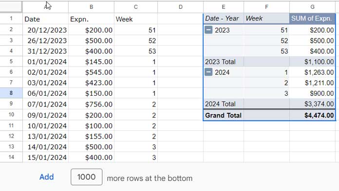
We have dates in column A and expenses in column B, where A1 and B1 contain the field labels ‘Date’ and ‘Expn.,’ respectively.

Let’s prepare this sample data suitable to group by week range in the Pivot Table.

a. Data Preparation Part

Firstly, enter the field label ‘Week’ in cell C1 and input the following formula in cell C2.

=ArrayFormula(LET(range, A2:A, n, (MAX(range)-MIN(range))/7, weeks, IFNA(HSTACK(SEQUENCE(n+1, 1, MIN(range), 7), IFERROR(SEQUENCE(n, 1, MIN(range)+6, 7), MAX(range))), MAX(range)), formatted, HSTACK(TEXT(SEQUENCE(ROWS(weeks)), "00."), TEXT(CHOOSECOLS(weeks, 1), "DD/MM/YYYY"), IF(CHOOSECOLS(weeks, 1), "-",), TEXT(CHOOSECOLS(weeks, 2), "DD/MM/YYYY")), weekrange, TRANSPOSE(QUERY(TRANSPOSE(formatted),, 9^9)), XLOOKUP(range, CHOOSECOLS(weeks, 1), weekrange, ,-1)))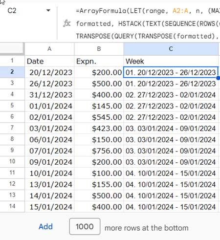

This formula converts dates to week ranges. It selects the dates in A2:A and converts them into week ranges in C2:C.

To adapt this formula to your date ranges, replace A2:A with the corresponding array references. Additionally, note that the date formatting is set to “DD/MM/YYYY.” You may need to change it to “MM/DD/YYYY” depending on your date formatting in A2:A.

You don’t need to learn this formula to proceed further. If you are particular about learning it, please check out this guide: Convert Dates to Week Ranges in Google Sheets (Array Formula).

Now, I suggest you remove all the empty rows below the data. Only add rows as and when required. This has three main benefits:

1. Improve the performance of your Sheet.
2. You don’t need to apply a Filter within the Pivot Table to exclude blank rows.
3. It keeps the formatting of the last row to the newly added row, which I’ve explained with images in one of my earlier guides here: How to Create Self-Formatting Tables in Google Sheets (With a Simple Initial Setup).

To remove rows below the last non-blank row in your Sheet, follow these steps:

1. Click on the first blank row below the data.
2. Press the Shift + Down arrow up to the last row in the Sheet.
3. Right-click any selected row.
4. Click on “Delete rows” in the context menu.

We have completed the data preparation part for grouping by week range in the Pivot Table in Google Sheets.

b. Grouping by Week Range in Pivot Table

This part is even simpler for most of you, as you may by now know that you need to group by the week range in column C and aggregate expenses. Here are those steps:

1. Click on Insert > Pivot Table.
2. Under “Data Range,” enter A:C.
3. Check “Existing Sheet” and click the cell in the current sheet or any other sheet where you want to create the Pivot Table. If you check “New Sheet,” Google Sheets will insert a new Sheet for the Pivot Table. I’m checking “Existing Sheet” and selecting cell E1.
4. Click “Create” to get the layout.
5. Add the field ‘Week’ to Rows and ‘Expn.’ to Values.

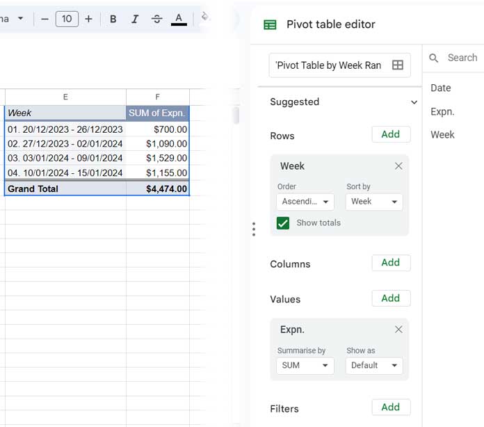
That’s it. This way, we can group by the week range in the Pivot Table in Google Sheets.

Group by Week Number in Pivot Table in Google Sheets

If your dates in column A do not spread across more than one year, you can simply replace the C2 formula in our previous example with the following formula to group by week number in a Google Sheets Pivot Table:

=ArrayFormula(IFERROR(WEEKNUM(DATEVALUE(A2:A), 1)))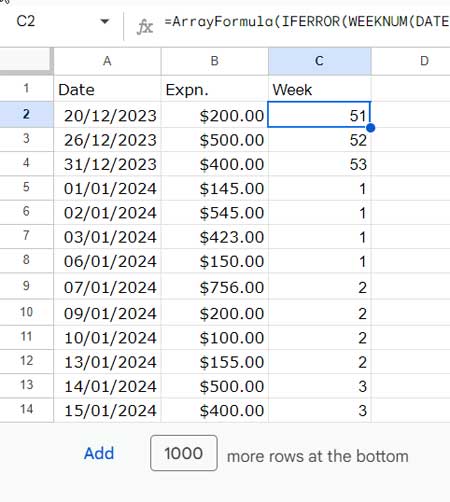

Note: The DATEVALUE in the formula prevents the WEEKNUM formula from considering a blank cell as 0 and returning a week number. As a result, WEEKNUM will return errors in blank cells, if any, and the IFERROR removes those errors.

In this formula, 1 represents that the week begins on Sunday and ends on Saturday. If you prefer a different starting day, please refer to the WEEKNUM function in my Date function guide: How to Utilize Google Sheets Date Functions (Complete Guide).

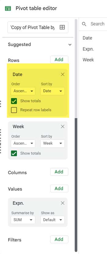
Whether your dates are spread across more than one year or not, I suggest you follow the below Pivot Table settings.

Add the ‘Date’ field on top of ‘Week’ within the Pivot Table editor panel.

Right-click on any date in the Pivot Table report, and select “Create pivot date group,” then “Year.”

This is the correct way to group by week number in the Pivot Table in Google Sheets.

Additional Tip: Aligning Group by Week Number and Week Range Results

Upon reviewing the output from both methods, you’ll notice that their results may not match. This discrepancy is expected since one method uses week ranges, and the other uses week numbers.

To align the results, follow these steps (to be applied to the Pivot Table that adopts grouping by week ranges):

In any blank cells, enter the following formula to find the Sunday prior to the lowest date in A2:A.

=MIN(A2:A)-WEEKDAY(MIN(A2:A))+1

Enter the date returned by this formula manually under the first non-blank cell in column A.

The Pivot Table is currently grouped by the week ranges in column C. Within the Pivot Table editor, add the ‘Date’ field above ‘Week.’

Then, right-click on any date in the Pivot Table report and select “Create pivot date group,” then “Year.”

Resources

1. How to Create a Weekly Summary Report in Google Sheets.
2. Query to Create Daily/Weekly/Monthly/Quarterly/Yearly Report Summary in Google Sheets.
3. Summarize Data by Week Start and End Dates in Google Sheets.