Google Sheets Pivot Tables don’t let you specify multiple values in the built-in Text contains or Text does not contain filters. The workaround is to use a custom formula with REGEXMATCH, allowing you to include or exclude multiple text values in a single condition.
This tutorial shows you exactly how to do that.
Formula Cheat Sheet
| Description | Formula |
|---|---|
| Multiple Conditions – Text Doesn’t Contain (Case Sensitive) | =REGEXMATCH(Attempt,"2nd|3rd")=FALSE |
| Multiple Conditions – Text Doesn’t Contain (Case Insensitive) | =REGEXMATCH(Attempt,"(?i)2nd|3rd")=FALSE |
| Multiple Conditions – Exact Match (Case Sensitive) | =REGEXMATCH(Attempt,"^2nd$|^3rd$")=FALSE |
| Multiple Conditions – Exact Match (Case Insensitive) | =REGEXMATCH(Attempt,"(?i)^2nd$|^3rd$")=FALSE |
Replace FALSE with TRUE to use Text contains instead of Text doesn’t contain.
Note: Enclose column names containing spaces in single quotes. For example, use 'Item No' instead of Item No.
Sample Data and Pivot Table
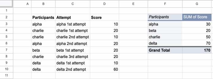
Suppose you have the following sample data in the range B2:D10.
| Participants | Attempt | Score |
|---|---|---|
| alpha | alpha 1st attempt | 10 |
| charlie | charlie 1st attempt | 20 |
| charlie | charlie 2nd attempt | 10 |
| alpha | alpha 2nd attempt | 20 |
| beta | beta 1st attempt | 20 |
| charlie | charlie 3rd attempt | 20 |
| delta | delta 1st attempt | 10 |
| delta | delta 2nd attempt | 60 |
Create a Pivot Table from the above data.
- Select the data.
- Click Insert > Pivot table.
- In the Pivot table editor, add Participants under Rows and Score under Values.
You will get a Pivot Table like the one below.
Now suppose you want to exclude rows where the Attempt field contains “2nd” or “3rd”. Notice that Attempt isn’t used in the Pivot Table itself.
The built-in Text does not contain filter only accepts a single value. For example, you can exclude 2nd or 3rd, but not both at the same time.
To filter multiple values, use a custom formula instead.
Multiple Values in Text Does Not Contain
To exclude rows containing 2nd or 3rd, use one of the following formulas in the Custom formula is field.
Case-sensitive
=REGEXMATCH(Attempt,"2nd|3rd")=FALSECase-insensitive
=REGEXMATCH(Attempt,"(?i)2nd|3rd")=FALSETo exclude more values, simply separate them with the pipe (|) operator.
2nd|3rd|4th|5thThe pipe symbol (|) acts as the OR operator in regular expressions. The above pattern matches 2nd, 3rd, 4th, or 5th.
How to Add the Custom Formula
- Click Add next to Filters in the Pivot table editor.
- Select the field to filter (Attempt in this example).
- Choose Filter by condition > Custom formula is.
- Paste one of the formulas above.
Using REGEXMATCH in a Pivot Table vs. a Worksheet
The formula used in the Pivot Table filter is slightly different from the one you would use in a worksheet.
For example, if you test the formula in a worksheet, you’ll need to use a range reference instead of the field name.
=ARRAYFORMULA(REGEXMATCH(C3:C10,"2nd|3rd"))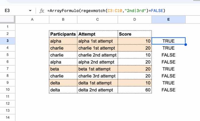
Keep these differences in mind:
- When using the formula in a worksheet, use the cell range (for example,
C3:C10) instead of the field name. - Since the reference is an array, wrap the formula with ARRAYFORMULA.
- Inside the Pivot Table editor, neither of these is required. You can simply use the field name (
Attempt).
REGEXMATCH returns TRUE when the text matches the specified pattern.
Since we want Text does not contain, we append =FALSE so matching rows are excluded.
Multiple Values in Text Contains
If you want to include only rows containing specific values, replace =FALSE with =TRUE.
=REGEXMATCH(Attempt,"2nd|3rd")=TRUEGoogle Sheets Pivot Table Filter Multiple Values Using Exact Match
The previous formulas perform partial matching (similar to Text contains and Text does not contain).
If you want to match only the exact text, use start (^) and end ($) anchors in the regular expression.
Partial match
2nd|3rd
(?i)2nd|3rd
Exact match
^2nd$|^3rd$
(?i)^2nd$|^3rd$
Replace 2nd and 3rd with the exact text values you want to match.
FAQ
Can I use multiple conditions in the built-in Text contains or Text doesn’t contain filter in a Google Sheets Pivot Table?
No. The built-in filter only supports a single condition. To filter by multiple values, use a REGEXMATCH formula in the Custom formula is field.
Can I use MATCH or XMATCH instead of REGEXMATCH?
Not for this use case. Both MATCH and XMATCH support the * and ? wildcards (XMATCH requires match_mode set to 2). However, the wildcard matching applies only to the search key, not the lookup values. Since we need to match the field value against multiple criteria, REGEXMATCH is the better choice.
Does the custom formula automatically include new rows added to the source data?
Yes. As long as the Pivot Table’s source range includes empty rows below the existing data before you apply the custom formula, newly added rows will be included automatically when the Pivot Table refreshes.
Conclusion
Although Google Sheets Pivot Tables don’t support filtering by multiple values using the built-in Text contains and Text does not contain conditions, you can achieve the same result with REGEXMATCH in a custom formula. By combining multiple values with the pipe (|) operator, you can easily include or exclude several text values in a single Pivot Table filter.
Related Tutorials
- How to Filter by Total in Google Sheets Pivot Tables
- How to Filter Top 10 Items in a Google Sheets Pivot Table
- Filter the Bottom 10 Items in a Pivot Table in Google Sheets
- Filter the Top 3 Values in Each Group in a Pivot Table – Google Sheets
- How to Sort and Filter Pivot Tables in Google Sheets (Complete Guide)
- How to Match Multiple Values in a Column in Google Sheets


Thank you for the tutorial. In your example, the field name is one word (i.e., “Attempt”). How do you address it when you have multiple words for the field name, for instance, “Material name” or “Number of units”? Range reference did not work for me. Thanks.
Specify them within single quotes.
E.g.:
=REGEXMATCH('All Attempts',"2nd|3rd")=FALSEHi Prashanth,
This is very helpful for me as well – many thanks.
i) I have to use a syntax with “;” instead of “,”, maybe because the sheet settings are “Locale = France” (this might address the remark made by nomwoyi Kunde on March 18, 2022).
ii) To EXCLUDE “2nd” and “3rd” attempts in the Pivot Table, I have to use the “FALSE” results of the regex (Filter applied to the “Attempt” column), i.e.:
=regexmatch(Attempt; "2nd|3rd") = FALSEIt works like a charm!
Best regards,
Thanks for your feedback.
Hello,
I’m following all the steps to use the custom filter, but it isn’t working.
Does the datasheet and pivot table have to be on the same page?
Hi, Enomwoyi Kunde,
Nope! Please check again. Also, you can leave the URL below (I will keep it unpublished)
Hi Prashanth,
This is very helpful – thanks.
Is there a way I can combine True and False in the same regexmatch formula? e.g. include “software” and exclude “SDR”
Thanks.
Ami
Hi, Ami Shimkin,
I may require an example to know what you are trying to do. From your question, I think FILTER may help.
Please feel free to share an example sheet link in the “Reply”.
Thanx for the reply. In my case, the data is on a different sheet so this won’t work.
I understand as of now it is probably not possible even with a script as filter views are not called through scripts.
I have already put a feature request many a time but so far it is not implemented.
But thanx anyway.
And you are really doing a good job.
I follow your post very diligently and find them very informative. I use the pivot table very extensively in my work.
I request if you can develop some script / some roundabout method to drill down to the filtered source data directly from the pivot table it would be a great help.
Presently the native feature creates a new sheet that is not of much use.
Hi, Srivastava,
Thanks for your feedback!
The similar thing you can achieve via Sheets’ new SLICERs. You can find that under the Data menu.
If your source data and the Pivot table are with in the same Sheet (same tab), you can filter your data and Pivot Table using this tool.
If the source and the Pivot table are in two different tabs, it won’t.
How to Use Slicer in Google Sheets to Filter Charts and Tables.
Here is one more related post – Drill Down Detail in Pivot Table in Google Sheets [Date Grouping]
Best,