You can filter a Google Sheets Pivot Table using various conditions. Among them, you can use Filter by Condition > Custom Formula to filter the top 10, 5, 3, or any number of values in each group in a Pivot Table.
Unlike Excel, Google Sheets does not provide a built-in “Value Filters” option for filtering the Top 10 values. This can make it challenging for beginners to filter the top 3 values by group in a Pivot Table.
However, by following my data settings, you can use a custom formula within the Pivot Table to achieve this.
Want to explore more advanced Pivot Table techniques? Check out our complete hub: How to Sort and Filter Pivot Tables in Google Sheets, covering top/bottom rankings, multi-level sorting, and flexible filtering options
Custom Formula to Filter the Top N Items in Each Group in a Google Sheets Pivot Table
=XMATCH(
   Category & Item,
   ArrayFormula(LET(
      qry, QUERY(QUERY(data, "SELECT Col2, Col1, SUM(Col3) WHERE Col2 IS NOT NULL GROUP BY Col2, Col1", 1), "OFFSET 1", 0),
      rnk, COUNTIFS(CHOOSECOLS(qry, 1), CHOOSECOLS(qry, 1), CHOOSECOLS(qry, 3), ">"&CHOOSECOLS(qry, 3))+1,
      FILTER(CHOOSECOLS(qry, 1)&CHOOSECOLS(qry, 2), rnk<=n)
   ))
)- data: The data range (columns: Item, Category, Value).
- Category & Item: Headers combined for matching.
- n: The number of values to retrieve (e.g.,
n=3for the top 3).
If 3, this formula filters the Pivot Table by the top 3 values in each group. For top 10, specify 10 instead.
Tie-Breaking Mode in Filtering the Top N Values in a Pivot Table
The custom formula follows the Excel Pivot Table interpretation: Highest N Values + Duplicates of the Nth Highest.
Example Data with Tie Handling
| Values | Included in Top 3 |
| 42 | ✅ |
| 42 | ✅ |
| 16 | ✅ |
| 16 | ✅ |
| 11 | ❌ |
| 10 | ❌ |
Explanation:
When applying a Top 3 filter, Excel includes all ties at the Nth position. The values 42, 42 are clearly in the top 3. The next highest value 16 is ranked 3rd, but since there is a tie at 16, both occurrences are included instead of arbitrarily excluding one. This approach ensures fairness in ranking.
Since rank positions determine filtering, we adopt the same logic in our custom formula.
Example: Filtering the Top 3 Items by Group in a Pivot Table in Google Sheets
Sample Data:
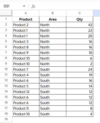
The goal is to create a Pivot Table that summarizes data by Area and Product and then filters the top 3 products in each region.
Steps to Create a Pivot Table:
- Select A1:C.
- Click Insert > Pivot Table.
- Choose New Sheet in the popup and click Create.
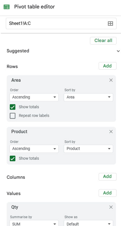
- Drag and drop Area and Product under Rows.
- Drag and drop Qty under Values.
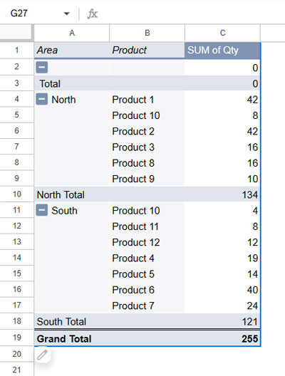
This will create a summarized Pivot Table. Since the data range contains empty rows, the Pivot Table may include an empty group, which can be ignored.
Applying the Custom Formula to Filter the Top 3 Items in Each Group
- Drag and drop Area under Filters.
- Click the filter dropdown and select Filter by Condition > Custom Formula Is.
- Copy-paste the following formula:
=XMATCH(
   Area & Product,
   ArrayFormula(LET(
      qry, QUERY(QUERY(Sheet1!A1:C, "SELECT Col2, Col1, SUM(Col3) WHERE Col2 IS NOT NULL GROUP BY Col2, Col1", 1), "OFFSET 1", 0),
      rnk, COUNTIFS(CHOOSECOLS(qry, 1), CHOOSECOLS(qry, 1), CHOOSECOLS(qry, 3), ">"&CHOOSECOLS(qry, 3))+1,
      FILTER(CHOOSECOLS(qry, 1)&CHOOSECOLS(qry, 2), rnk<=3)
   ))
)- Click OK.
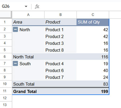
This will filter the top 3 items in each group within the Pivot Table.
Breakdown of the Formula:
qry:
QUERY(Sheet1!A1:C, "SELECT Col2, Col1, SUM(Col3) WHERE Col2 IS NOT NULL GROUP BY Col2, Col1", 1)- Groups the data by Area and Product, summing the Qty.
QUERY(..., "OFFSET 1", 0)- Removes the header row from the first query result.
rnk:
COUNTIFS(CHOOSECOLS(qry, 1), CHOOSECOLS(qry, 1), CHOOSECOLS(qry, 3), ">"&CHOOSECOLS(qry, 3))+1- Returns the group-wise ranking of each item.
Final Filtering Expression:
FILTER(CHOOSECOLS(qry, 1)&CHOOSECOLS(qry, 2), rnk<=3)- Filters the Area & Product wherever the rank ≤ 3.
XMATCH:
XMATCH(Area&Product, ...)- Matches the filtered Area & Product and returns the relevant rows.
Conclusion
By using this custom formula, you can effectively Filter the Top 3 Values in Each Group in a Pivot Table in Google Sheets. This method replicates Excel’s behavior while handling ties efficiently.


