


Assume 50, 49, 48 are the top 3 scores in a cricket match. But two batsmen have scored 48 runs each. Then how to get the scores 50, 49, 48, and 48 when extracting top 3 scores? To filter top n values including duplicates in Google Sheets, you can use SORTN.
With the help of a SORTN formula, Google Sheets users can extract top or bottom n values in Google Sheets. In concise, use this tutorial to get to know;
- How to extract or filter to a new range top 3, 5, 10 or n values including duplicates in Google Sheets.
- Extracting or filtering to a new range bottom 3, 5, 10, or n values including duplicates in Google Sheets.
Let’s begin with the following sample dataset to extract top n values with duplicates.
Sample Data to Filter to a New Range Top N Values with Duplicates
(Student Names and Their Marks out of 50 in an Exam)
| A | B | |
| 1 | Roger | 50 |
| 2 | Johnny | 48 |
| 3 | Patricia | 48 |
| 4 | Martha | 47 |
| 5 | David | 46 |
| 6 | Jonathan | 45 |
| 7 | Theresa | 40 |
| 8 | Ruby | 38 |
| 9 | Linda | 29 |
| 10 | Susan | 29 |
| 11 | Jennifer | 25 |
| 12 | Louis | 24 |
Here do you want the top n marks only or top n marks with the student names?
For example, if you want to extract the top 5 marks, the result would be the marks 50, 48, 48, 47, 46, and 45.
Note: If you count these values, you will get 6 instead of 5 as there is one duplicate mark in the top 5 ranks.
If you want to extract the names too with the marks, the result would be like;
| C | D | |
| 1 | Roger | 50 |
| 2 | Johnny | 48 |
| 3 | Patricia | 48 |
| 4 | Martha | 47 |
| 5 | David | 46 |
| 6 | Jonathan | 45 |
I have solutions for both the above scenarios. Here we go!
SORTN to Extract Top N Values Including Duplicates in Google Sheets
As the title suggests, the formula here is based on SORTN. To get only the top 5 values (of course that including duplicates), use the below SORTN formula.
=sortn(B2:B13,5,3,1,0)In this SORTN formula, B2:B13 is the range containing the marks of the students. The number 5 represents n.
That means to filter top 10 values including duplicates to a new range, change 5 to 10.
=sortn(B2:B13,10,3,1,0)What about extracting top 10 values including duplicates and corresponding names? Here is that SORTN formula.
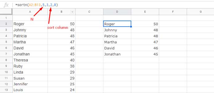
=sortn(A2:B13,5,3,2,0)Here in the formula, I have just included the range that contains the names too. In addition to that changed the sort column to 2 (the column index number containing the marks). The sort column is the fourth argument in the formula.
This way you can extract top 5, top 10, top n values including duplicates in Google Sheets.
Extract Bottom N Values Including Duplicates in Google Sheets
In rare cases, depending on your nature of the job assigned, you may require a formula to filter/extract bottom 5, 10 or n values. Don’t worry! The above SORTN formula will come in handy in this case too.
To extract bottom n values, including duplicate values, use the following formula.
=sortn(A2:B13,5,3,2,1)Just compare this formula with the last formula. What changes do you see?
The change in only in the last argument. Earlier it was the value 0 now it’s 1. Actually it’s sort order.
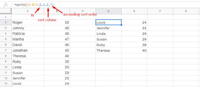
To filter/extract top n numbers with duplicates, I have sorted the data (numeric column) in descending order.
To get bottom n values, we should sort the data (numeric column) in ascending order. That’s what we have done in the last formula.
Conclusion
In Excel, you might have seen or used a different approach to get top or bottom n values with duplicates.
Why didn’t you see such a smarter solution using SORTN in Excel? My guess, Microsoft has introduced SORTN only in the latest iterations of Excel.
Want to apply the above logic in a Pivot Table in Google Sheets? Then do follow this guide – How to Filter Top 10 Items in Google Sheets Pivot Table.
That’s all for now! Hope you have enjoyed the stay here.
What does the 3 mean in the parentheses?
It’s display_ties_mode.