
It’s impossible to list every custom formula rule you can use in data validation because there is no limit. What matters is understanding how custom formulas work in data validation. Once you understand them, you can use many of your existing Google Sheets formulas to build custom validation rules.
How the Custom Formula Differs from Built-in Rules
Google Sheets provides several built-in data validation rules. Built-in validation rules work well for most situations. However, they validate only the value in the cell being edited. When your rule depends on another cell or requires more complex logic, use Custom formula is.
For example, you can’t allow data entry in one cell only when another cell contains a value. For such validation rules, Custom formula is is the only option.
Cell References in Custom Formula Data Validation
Similar to custom formulas in conditional formatting, relative and absolute references also play a key role in data validation.
The success of a custom formula often depends on using the correct cell reference. The following table summarizes how each reference type behaves.
| Reference | Type | Changes When Applied | Common Use |
|---|---|---|---|
A1 | Relative | Row and column change | Validate each cell based on its own value. |
$A$1 | Absolute | Neither row nor column changes | Use one control cell for the entire validation range. |
$A1 | Mixed | Row changes, column fixed | Validate a cell using a value in the same row. |
A$1 | Mixed | Column changes, row fixed | Validate cells based on column headers. |
Understanding these reference types is essential for building effective custom validation rules.
Syntax
The syntax of the Custom formula is rule is:
=formula_returning_TRUE_or_FALSEThe formula is evaluated for every cell in the validation range.
Example:
=COUNTIF($A$2:$A$10, A2)=1This formula allows only unique values by rejecting duplicate entries.
A custom formula must return TRUE to accept the input and FALSE to reject it.
When to Use a Custom Formula
Use Custom formula is when the built-in data validation rules aren’t enough. Typical use cases include:
- Validating a cell based on the value in another cell, either on the same sheet or a different sheet in the workbook.
- Allowing only specific text patterns.
- Preventing duplicate entries in Google Sheets.
- Creating multi-row dynamic dependent drop-downs.
- Restricting input based on dates, weekdays, or other conditions.
Custom Formula Examples in Data Validation
To understand relative and absolute references in data validation, let’s go through four examples.
Example 1: Relative Reference (A1)
In many cases, the built-in data validation rules are sufficient. However, when you need more complex validation, you must use a custom formula.
For example, the custom formula used in my Word Guess Game enforces multiple rules, such as:
- Allow only one letter per cell.
- Prevent players from skipping rows.
- Require players to reveal at least one clue before unlocking the next row.
The following example shows why a relative reference is required.
Assume you have an attendance sheet, and you want to allow only the attendance codes P, A, H, SL, EL, PL, and CL in the range B2:E8.
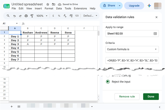
- Select B2:E8.
- Click Data > Data validation > Add rule.
- Under Criteria, select Custom formula is.
- Enter the formula:
=OR(B2="P", B2="A", B2="H", B2="SL", B2="EL", B2="PL", B2="CL")- Expand Advanced options and select Reject the input.
- Click Done.
The cell reference B2 is a relative reference. As the validation rule is applied across the range, Google Sheets automatically adjusts it for each cell. For example, the formula checks C2 in cell C2, D5 in cell D5, and E8 in cell E8.
If you enter a value other than the specified attendance codes, the rule rejects the input and displays the following warning:
There was a problem
The data that you entered in cell B2 violates the data validation rules set on this cell.
Example 2: Absolute Reference ($A$1)
Assume the range A2:A5 contains the labels Name, Age, City, and Country. Allow data entry in B2:B5 only when cell B1 is set to Yes.
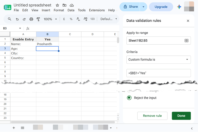
You can apply the following custom formula to the range B2:B5.
=$B$1="Yes"Every cell in B2:B5 checks the same cell (B1).
When B1 is not Yes, Google Sheets rejects any new entries in B2:B5.
Note: If you want to control only a single cell, select B2 instead of B2:B5 before creating the validation rule.
This technique is useful in templates. For example, you can prevent accidental data entry by using a checkbox or a Yes/No switch to temporarily enable or disable a range. Although Google Sheets also provides Protect sheets and ranges, this method makes it easy to open and close input ranges without changing protection settings.
Example 3: Mixed Reference ($A1)
Assume the range A2:A5 contains student names. Allow users to enter scores in B2:B5 only when the corresponding student name is not blank.
Apply the following custom formula to the range B2:B5:
=$A2<>""The column reference (A) is fixed, while the row reference changes automatically. Google Sheets evaluates the formula like this:
- B2 checks A2.
- B3 checks A3.
- B4 checks A4.
- B5 checks A5.
If you also want to apply the same rule to other columns, simply change the validation range from B2:B5 to B2:E5 (or any wider range). Each cell will continue checking the name in column A of the same row.
Example 4: Mixed Reference (A$1)
Assume item names are in A2:A5, and weekday names are in B1:H1.
Allow data entry only in weekday columns and prevent entry in the Saturday and Sunday columns.
Select the range B2:H5 and apply this custom formula:
=NOT(OR(B$1="Sat",B$1="Sun"))The row reference (1) is fixed, while the column reference changes automatically. As the rule is applied across the range, it checks the corresponding column header:
- B2 checks B1.
- C2 checks C1.
- D2 checks D1.
- and so on.
The formula first checks whether the column header is Sat or Sun. If so, OR returns TRUE. The NOT function reverses that result, allowing data entry only in weekday columns.
FAQ
Can I apply multiple custom formulas (data validation rules) to the same cell?
No. You can apply only one data validation rule to a cell or range.
For example, a drop-down list and a checkbox are both data validation rules. If a cell already has one of these rules, you can’t apply another built-in rule or a custom formula on top of it.
If you need multiple conditions, combine them into a single custom formula using functions such as AND, OR, or NOT.
How do I refer to a cell on another sheet in a data validation custom formula?
This is a common source of confusion because conditional formatting requires the INDIRECT function when referring to a cell on another sheet.
However, in a data validation custom formula, you can refer to a cell on another sheet directly by including the sheet name. For example:
=Sheet1!$B$1="Yes"If the sheet name contains spaces, enclose it in single quotes:
='Employee List'!$B$1="Yes"No INDIRECT function is required.
Can I use functions like VLOOKUP, XLOOKUP, FILTER, or QUERY in a custom formula?
Yes, as long as the formula ultimately returns TRUE or FALSE. If it returns another value, wrap it in a logical test.
Why does my custom formula reject all input?
Common reasons include:
- incorrect relative or absolute references
- formula returns text instead of TRUE/FALSE
- validation applied to the wrong range
- referenced cells are blank
Conclusion
Once you understand how relative, absolute, and mixed references behave, creating custom validation rules becomes much easier. You can combine this knowledge with functions such as AND, OR, NOT, COUNTIF, MATCH, and REGEXMATCH to build powerful validation rules for almost any scenario.
If you want to learn more about data validation rules, custom formulas, and other tips, check out The Complete Guide to Data Validation in Google Sheets.