In this tutorial, I’ll share a practical Google Sheets tip for formatting the QUERY Pivot Header Row in a simple and reliable way.
Formatting QUERY pivot headers is a common requirement, but many users struggle to find an effective solution. In practice, I often see formulas made unnecessarily complex when trying to solve this problem.
Instead, this tutorial uses a different approach to format the header row in the output of a QUERY pivot—by leveraging the TRANSPOSE function. This method keeps the formula clean while giving you full control over the header formatting.
You can apply this technique to QUERY pivot headers containing dates, times, or numeric values.
Part of the QUERY Pivot & Reporting in Google Sheets series, this tutorial explains how to format QUERY pivot headers when direct formatting is not supported.
1. How to Format the QUERY Pivot Header Row Containing Dates
Example:
Let’s use a small dataset in A2:C8 with three columns: Date (Column A), Description (Column B), and Amount (Column C). Row 2 (A2:C2) contains the headers.
Here’s a basic Pivot Table using the QUERY function in Google Sheets:
=QUERY(A2:C8, "SELECT B, SUM(C) GROUP BY B PIVOT A")
In this case, the header row contains dates because the Pivot column is A. Can you format this pivot column using the FORMAT clause as follows?
You might want to convert the header row dates from the format YYYY-M-D to DD/MMM/YYYY.
Incorrect Formula:
=QUERY(A2:C8, "SELECT B, SUM(C) GROUP BY B PIVOT A FORMAT A 'DD/MMM/YYYY'")This formula won’t work and will return a #VALUE! error.
Unfortunately, Google Sheets doesn’t support formatting the QUERY Pivot Header Row with the FORMAT clause. So, how can you format the header row in the QUERY Pivot output?
Steps
- Interchange the Group Column with the Pivot Column.
This is the critical step.
Instead of pivoting Column A, pivot Column B, and group Column A (according to the example dataset above).
The formula becomes:=QUERY(A2:C8, "SELECT A, SUM(C) GROUP BY A PIVOT B") - Format the Grouped Column.
You can now format the Grouped Column using the FORMAT clause.=QUERY(A2:C8, "SELECT A, SUM(C) GROUP BY A PIVOT B FORMAT A 'DD/MMM/YYYY'") - Transpose the Result.
Finally, transpose the output to flip the headers into rows:=TRANSPOSE(QUERY(A2:C8, "SELECT A, SUM(C) GROUP BY A PIVOT B FORMAT A 'DD/MMM/YYYY'"))

This way, you’ve effectively formatted the header row in your Google Sheets QUERY Pivot formula!
2. Format Numbers and Time in the QUERY Pivot Header
You can use the same approach outlined above to format numbers and time in the QUERY Pivot header.
To explore the available formats for dates, times, and numbers in QUERY, check out How to Format Date, Time, and Number in Google Sheets QUERY.
3. How to Format the QUERY Pivot Header Row Containing Month Numbers
Here’s a practical tip on formatting month numbers in the QUERY Pivot Header row to display as month names in text format.
In this example, we group by item descriptions and pivot by the month number, resulting in the month numbers appearing in the header row.
=QUERY(A2:C8, "SELECT B, SUM(C) GROUP BY B PIVOT MONTH(A)")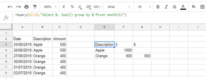
Here’s how you can convert these month number headers into month names in text format.
This technique builds on the same date-conversion logic explained in Google Sheets Query: How to Convert Month Number to Month Name (Text).
What if we don’t group by month numbers directly? What’s the alternative?
We’ll adapt the approach from Example #1, making slight modifications to achieve the desired result.
Previous Approach (Example #1):
- Group by the Date column.
- Pivot by the Text column.
- Format the Date column.
- Transpose the output.
This method doesn’t work well for month numbers because the pivot column treats numbers differently than date formatting.
New Approach:
- Convert dates in the Date column to beginning-of-month dates.
- Group by this new Date column.
- Pivot the Text column.
- Format the new Date column.
- Transpose the result.
Instead of grouping by the month number, group by the beginning-of-month dates. This ensures all dates within a month are grouped under one single date (e.g., the 1st of the month). Format this date to display the month in text format (e.g., “MMM”).
To implement this, ensure the data is well-structured, rather than simply specifying A2:C8 as in earlier examples.
Formula for Data Preparation:
=ArrayFormula(HSTACK(VSTACK(A2, IFERROR(EOMONTH(DATEVALUE(A3:A8), -1)+1)), B2:C8))You should use this as the ‘data’ in the QUERY formula.
Formula Breakdown:
DATEVALUE(A3:A8): Converts the dates in range A3:A8 to actual date values. If a cell is blank, it generates an error, avoiding issues with defaulting to30/12/1899(serial number 0).EOMONTH(..., -1): Finds the end of the previous month for each date.+1: Moves to the first day of the following month (beginning of the month).IFERROR(...): Replaces errors (e.g., from blank cells) with blanks.VSTACK(A2, ...): Stacks the header value in A2 on top of the calculated beginning-of-month values.HSTACK(..., B2:C8): Horizontally combines the processed date column with columns B and C.
Final QUERY Formula:
=TRANSPOSE(QUERY(ArrayFormula(HSTACK(VSTACK(A2, IFERROR(EOMONTH(DATEVALUE(A3:A8), -1)+1)), B2:C8 )), "SELECT Col1, SUM(Col3) GROUP BY Col1 PIVOT Col2 FORMAT Col1 'MMM-YYYY'"))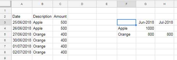
Key Notes:
- The QUERY formula uses Col1, Col2, and Col3 as column identifiers because the data is virtual and not directly in the spreadsheet.
- Replace
'MMM-YYYY'in the FORMAT clause with your desired date format (e.g.,'MMM'for abbreviated month names or'MMMM'for full month names).
Final Notes
Formatting the header row in a QUERY pivot requires working around a known limitation in Google Sheets: pivot headers cannot be formatted directly using the FORMAT clause.
By rearranging the GROUP BY and PIVOT columns and transposing the result, you can apply standard QUERY formatting rules to the header row in a controlled and reliable way. This approach works consistently for dates, times, numbers, and even derived values such as month-based headers.
Once you understand this pattern, formatting QUERY pivot headers becomes predictable and reusable—making QUERY pivots far more suitable for structured reports and dashboards.
For more techniques related to controlling layout, ordering, totals, and formatting in QUERY pivots, refer to the QUERY Pivot & Reporting in Google Sheets series.


How about there are two or more items in the Group clause instead of 1 column B?
Hi, An Dang,
In that case, the above tips won’t work. You should format the data before processing with Query.
E.g.:
Formula as per the tutorial:-
=transpose(query(A2:C8,"Select A, Sum(C) group by A Pivot B format A'dd/mmm/yyyy'"))Recommended:-
=ArrayFormula(query({text(A2:A8,"dd/mmm/yyyy"),B2:C8},"Select Col2, Sum(Col3) group by Col2 Pivot Col1"))In the second one, you can group by two or more columns.
Million thanks, this is a direct way, no need to work around with the transpose.
What if we want to sort the Query Pivot Header from the farthest day to the nearest day. Could you help?
Hi, An Dang,
For that, you may please try the below syntax.
=transpose(query(transpose(query_formula),"select * order by Col1 desc"))You can also try the built-in pivot table (Insert > Pivot table), which has the said feature.
THANKS A LOT!! 🙂