You can separate your data into small chunks in many ways: One way is to create new tables for each category, and another option is to divide the data into equally sized small tables.
This tutorial explains how to split your Google Sheet data into category-specific tables. If you’re interested in dividing it into equal-sized sections, check out this tutorial: Dynamic Formula – Split a Table into Multiple Tables in Google Sheets.
Sample Data and Expected Results
The provided sample data comprises four columns: Date, Item, Category, and Amount, denoted as columns A to D.
Sample Data:
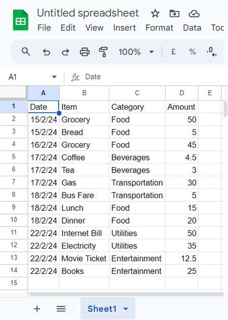
There are five distinct categories listed under the “Category” column: Food, Beverages, Transportation, Utilities, and Entertainment.
Upon splitting the sample data into category-specific tables, five tables will be generated.
Expected Results:
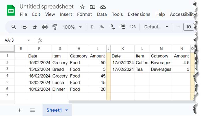
Note: The screenshot displays only a portion of the result since it’s not feasible to show all five tables on one screen. To view the complete result in real time, you can utilize the template provided below.
We can address this task of splitting into category-specific tables using two methods. The first method involves using multiple FILTER functions, employing one for each category. The second method employs a dynamic approach, combining REDUCE and FILTER. Both approaches will be explored.
Organize Data into Category-Specific Tables Using the FILTER Function
Steps:
In cell F2, input the following combination of TOCOCL and UNIQUE to obtain unique categories without blanks:
=TOCOL(UNIQUE(C2:C), 1)In cell G1, apply the following FILTER formula to filter the first category, which is “Food”:
=VSTACK($A$1:$D$1, FILTER($A$1:$D, $C$1:$C=$F$2))Explanation:
=VSTACK($A$1:$D$1, …)– vertically appends the header row with the filtered results.FILTER($A$1:$D, $C$1:$C=$F$2)– filters the dataset based on the category column, specifically where the category matches the value in cell F2.
Copy and paste this formula into the first cell of a different range, for example, cell L1, and replace $F$2 with $F$3. Repeat the same.
This semi-automatic approach enables you to split your data into category-specific tables in Google Sheets.
Split Google Sheet Data into Category-Specific Tables Using FILTER and REDUCE Combo
In the earlier example, we used the UNIQUE and TOCOL combination to retrieve the unique categories. We employed the values in that array (criteria range) as the criteria within multiple FILTER formulas.
In this scenario, we use a single FILTER formula within REDUCE and employ REDUCE to iterate over each element in the criteria range within the FILTER criteria.
The result in each filter will be horizontally stacked.
Formula:
=REDUCE(
   TOROW(, 1),
   TOCOL(UNIQUE(C2:C), 1),
   LAMBDA(accumulator, value,
      IFNA(HSTACK(accumulator,
         VSTACK(A1:D1, FILTER(A1:D, C1:C=value)),
      ))
   )
)
Please scroll up to view the screenshot of the expected result, where I’ve used this formula in cell F1.
Before explaining how the formula splits Google Sheets data into category-specific tables, here is the syntax of the REDUCE function.
Syntax:
REDUCE(initial_value, array_or_range, lambda)Formula Explanation
initial_value: TOROW(, 1) – To illustrate, let’s consider an example where cell A1 is blank. If you use TOCOL(A1, 1), the formula returns any value, excluding empty cells. Since A1 is empty, the formula merely removes it. TOROW(, 1) is equivalent to the same.array_or_range: TOCOL(UNIQUE(C2:C), 1) – Represents the unique categories in the table.LAMBDA(accumulator, value, …)– This defines a lambda function with two arguments:accumulator: Holds the intermediate result accumulated so far by the REDUCE function. Theinitial valuewithin it is the output of TOROW(, 1).value: Represents the current unique value from thearray_or_range.
Here is the function in use:
IFNA(HSTACK(accumulator, VSTACK(A1:D1, FILTER(A1:D, C1:C=value)), ))- The IFNA function handles #NA errors that may occur when stacking unequal-sized arrays.
- HSTACK function: Horizontally stacks the
accumulatorvalue with the VSTACK and FILTER combination, followed by a blank cell (indicated by the comma immediately after the said combination). The VSTACK appends the header row on top of the FILTER result. - FILTER formula: Filters the range A1:D based on C1:C matching
value.
Conclusion
The REDUCE function simplifies the process of merging and combining data in Google Sheets. Splitting data into category-specific tables is just one example of its versatility.
Likewise, we can utilize REDUCE to combine multiple sheets within a workbook or merge tables in Google Sheets. Here are some related resources.
- How to Left Join Two Tables in Google Sheets
- How to Right Join Two Tables in Google Sheets
- How to Inner Join Two Tables in Google Sheets
- How to Full Join Two Tables in Google Sheets
- Master Joins in Google Sheets (Left, Right, Inner, & Full) – Duplicate IDs Solved
- Dynamically Combine Multiple Sheets Horizontally in Google Sheets
- Combine Data Dynamically in Multiple Tabs Vertically in Google Sheets


