With the assistance of a dynamic formula, we can split table or formula result ranges into multiple tables in Google Sheets. The user needs to specify the row size of the tables.
For instance, if you specify 15 (row size) and the table contains 50 rows, you will have 4 tables, with the first three tables containing 15 rows each and the fourth table containing 5 rows.
We will utilize the REDUCE lambda function for this operation. However, it is a resource-intensive function. If you encounter any issues, I can provide an alternative option that is simpler, although it requires using multiple formulas – one formula per table.
Splitting a Table into Multiple Tables: Why Is It Useful?
When you divide a table into multiple tables, the formula positions the tables side by side, leaving a blank column between them.
This is advantageous when printing tables, as it minimizes the number of pages needed for the entire table. However, this may not be applicable if your table has numerous columns.
Additionally, it facilitates easier navigation. Breaking down tables into smaller sections simplifies the process of locating specific data and concentrating on pertinent information.
Prerequisites
The formula that dynamically splits a table into multiple tables requires a closed range when using physical data for splitting, not an open range.
For example, you can specify A2:C100, not just A2:C, in the formula. If you have a growing table, consider using the range as follows: FILTER(A2:C, A2:A<>""), as this will accommodate future ranges.
Exclude the header row of the table. If your table is in A1:F50 and A1:F1 contains field labels, use the range A2:F50 or FILTER(A2:F, A2:A<>""), excluding the header row.
How to Split a Table into Multiple Tables in Google Sheets
Below is a dynamic formula for splitting a table into multiple tables in Google Sheets.
=LET(data, range, n, rows, t_size, ROWS(CHOOSECOLS(data, 1)),
   base, SEQUENCE(1, ROUNDUP(t_size/n), 1, n),
   header, HSTACK("label1", "label2, ..."),
   REDUCE(TOROW(, 1), base, LAMBDA(a, v, IFERROR(
      HSTACK(a,
         VSTACK(
            header,
            FILTER(data, ISBETWEEN(SEQUENCE(t_size), v, v+n, TRUE, FALSE))
         ),
      )
   )))
)
Make the following adjustments in the formula to tailor it to your table:
- Replace
rangewith the actual table range, for example, A2:C100 orFILTER(A2:C, A2:A<>""). - Replace
rowswith the desired number of rows for each split table, for instance, 10. - Additionally, modify the headers within the HSTACK function based on your table’s structure. If your table has four columns, adjust it as
HSTACK("label1", "label2", "label3", "label4"). Substitute the placeholder texts with the actual field names.
Example of Splitting a Table into Multiple Tables Using a Dynamic Formula
We have a dynamic formula and instructions to split a table into n tables in Google Sheets. Let’s test it with a small sample dataset that contains three columns and 17 rows. The table range is A2:C18.
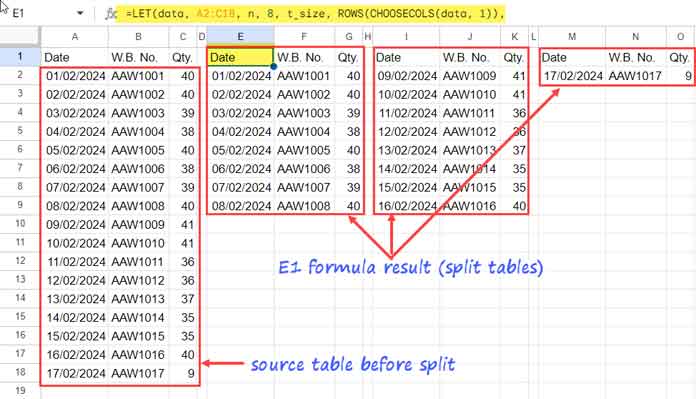
We will split this table into multiple tables, each having 8 rows. Consequently, there will be three tables, with the first two tables containing 8 rows each, and the last table containing 1 row. Additionally, these tables will have an additional header row.
Formula:
=LET(data, A2:C18, n, 8, t_size, ROWS(CHOOSECOLS(data, 1)),
   base, SEQUENCE(1, ROUNDUP(t_size/n), 1, n),
   header, HSTACK("Date", "W.B. No.", "Qty."),
   REDUCE(TOROW(, 1), base, LAMBDA(a, v, IFERROR(
      HSTACK(a,
         VSTACK(
            header,
            FILTER(data, ISBETWEEN(SEQUENCE(t_size), v, v+n, TRUE, FALSE))
         ),
      )
   )))
)
Notes:
- If your source table includes a date or timestamp column, the resulting table may contain date values in the corresponding columns. To address this, select those columns and apply the date format. To do so, once selected, click on Format > Number > Date or Date time.
- Any changes made in the source table will be reflected in the results.
- You have the flexibility to replace physical ranges with formula outputs, such as QUERY, FILTER, SORT, etc. To implement this, replace the
rangewith the formula itself. In the above example, you can replace A2:C18 with a QUERY or other formulas that return an array result. Ensure that the formula results do not contain a header.
Formula Breakdown
You don’t need an in-depth understanding of the formula to use it for splitting a table into multiple equal-sized tables. The formula involves Lambda, which might be a bit challenging for new users to comprehend.
However, if you have some basic knowledge of lambda functions, particularly REDUCE, you may find the breakdown of the formula below worth reading.
The LET function is utilized to code the formula, assigning names to value expressions and returning the result of the formula expression.
Syntax:
LET(name1, value_expression1, [name2, …], [value_expression2, …], formula_expression)Value Expressions and Names:
There are five value expressions with assigned names in the formula. They are as follows:
A2:C18: Represents the source table, anddatais the assigned name.8: Represents the number of rows in each table, andnis the assigned name.ROWS(CHOOSECOLS(data, 1)): Returns the total number of rows in the source table, with the assigned namet_size.SEQUENCE(1, ROUNDUP(t_size/n), 1, n): Generates an array, assigned the namebase. It plays a key role in the formula expression. Let me elaborate on what it returns and its purpose.- In the given example, with real values, the
basewill beSEQUENCE(1, ROUNDUP(17/8), 1, 8), resulting in the array{1, 9, 17}. These numbers represent corresponding rows in the source table, serving as the first rows in the new tables.ROUNDUP(17/8)equals 3, indicating there will be three tables after the split, where 17 is the total number of rows in the source table, and 8 is the number of rows required in each split table.- The SEQUENCE function generates 3 numbers starting from 1, with a step of 8. Thus, the result will be
{1, 9, 17}.
- In the given example, with real values, the
HSTACK("Date", "W.B. No.", "Qty."): Represents the headers of the split table, andheaderis the assigned name.
Formula Expression:
REDUCE(TOROW(, 1), base, LAMBDA(a, v, IFERROR(
      HSTACK(a,
         VSTACK(
            header,
            FILTER(data, ISBETWEEN(SEQUENCE(t_size), v, v+n, TRUE, FALSE))
         ),
      )
   )))
Explanation:
The REDUCE function operates with an initial value and an array, applying a lambda function to each element and accumulating the results.
- The initial value is set as
TOROW(, 1), which is equivalent toTOROW(A1, 1)considering A1 is empty. Using 1 in the second argument of the TOROW function, ensures compatibility with potential empty cells, preventing the return of blanks. - The array specified is
base, containing{1, 9, 17}. This array determines the values over which the REDUCE function iterates, applying the specified lambda function to each element ofbase. - The lambda function takes two parameters,
arepresenting the accumulator, initially set asTOROW(, 1), andvrepresents the current element in the array. - The core of the formula lies in the lambda function, where HSTACK and VSTACK functions are used to horizontally and vertically stack arrays, respectively.
The FILTER formula, i.e., FILTER(data, ISBETWEEN(SEQUENCE(t_size), v, v+n, TRUE, FALSE)), filters the source data based on row numbers between v (inclusive) and v+n (exclusive), as described in the reference to the ISBETWEEN function.
For example, when v is 1 and v+n is 9, the formula filters records in the table from rows 1 to 8. This filtered data is then vertically stacked with the header row using VSTACK.
The HSTACK function combines the current accumulator value a with the stacked data and introduces a blank cell:
HSTACK(a, VSTACK(header, FILTER(data, ISBETWEEN(SEQUENCE(t_size), v, v+n, TRUE, FALSE))), )The REDUCE function iterates through the base array, applying the lambda function each time. The final result is the concatenation of filtered and stacked tables, with #N/A errors removed using IFERROR.
For example, with ‘base’ {1, 9, 17}, it filters data from rows 1 to 8, then 9 to 16, and finally 17 to 24. These filtered tables are stacked horizontally with blank cells separating each split table. The IFERROR function ensures any #N/A errors that might arise during the stacking process are removed from the final result.
Split a Table into Multiple Tables Using QUERY: Non-Dynamic, But Better Performance
If you encounter issues with the dynamic formula due to a large volume of data for column splitting, consider using the following QUERY formula option. This is the easiest way to split a table into multiple tables in Google Sheets.
Assuming the table range is A1:C18 with A1:C1 containing field labels, and you want 8 rows per table, use the following formula in cell E1:
=QUERY($A$1:$C, "SELECT * WHERE Col1 IS NOT NULL LIMIT 8 OFFSET 0", 1)Unlike the dynamic formula, you can use an open range A1:C; it’s not necessary to specify a closed range like A1:C18. Also, you can include headers in the range, unlike the dynamic formula where we used A2:C18.
The QUERY formula selects all columns where column 1 is not null, excluding blank rows based on column 1, and limits the output to 8 rows. There is no offset from the beginning of the table.
Copy this formula and paste it into I1, replacing OFFSET 0 with OFFSET 8. Then paste the formula into M1, replacing OFFSET 0 with OFFSET 16. It’s that simple.
Conclusion
This post explores two distinct approaches to splitting a table into multiple equal-sized tables side by side in Google Sheets. I prefer the dynamic approach as it autonomously handles the creation of new tables.
When employing the dynamic formula, consider using FILTER with the range, such as replacing A2:C18 with FILTER(A2:C, A2:A<>"). This offers the advantage that as your source table expands, the formula will autonomously create new tables.
While QUERY is also a viable option in Google Sheets, it is non-dynamic and requires user interaction.
Before concluding, one more thing to note: if you are interested in joining tables instead of splitting them, I have already provided tutorials on that. Please refer to the resources below:


