The UNIQUE function in Google Sheets is case-sensitive by default. However, there are a few effective ways to achieve case-insensitive uniqueness.
Typically, users combine the functions PROPER, LOWER, or UPPER with UNIQUE to create case-insensitive results. However, this approach has a small drawback: it converts the returned output to the chosen case (proper, lower, or upper).
Here’s the formula syntax:
=ArrayFormula(UNIQUE(PROPER(range)))You can swap PROPER with LOWER or UPPER.
Below, I’ve demonstrated how these combinations work by converting a few food and dish names in the range A2:A5.
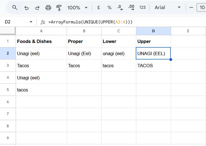
In this example, the second column uses the formula:
=ArrayFormula(UNIQUE(PROPER(A2:A5)))The third and fourth columns replace PROPER with LOWER and UPPER, respectively.
The output should be “Unagi (eel)” and “Tacos” as the first occurrences of the case-insensitive unique values, without altering the case of the original values.
Interestingly, if you use =UNIQUE(A2:A5) in Excel, it returns the expected result since the UNIQUE function in Excel is case-insensitive. How can we achieve the same result in Google Sheets, i.e., without altering the case of the original values in the range (A2:A5)?
Case-Insensitive Unique Values Without Altering Case
Here are my three best suggestions for achieving case-insensitive unique values in Google Sheets. The first two formulas use running counts to return unique values, while the third formula uses the REDUCE function for case-insensitive uniqueness.
Why is the third formula interesting?
The REDUCE function is typically used to reduce an array into a single value, but in this case, the reduced value can even be an array containing multiple values.
Let’s dive into the formulas.
Formula Option #1:
=FILTER(A2:A, COUNTIFS(A2:A, A2:A, ROW(B2:B), "<="&ROW(A2:A)) = 1)The COUNTIFS function generates a running count of the values in the range A2:A. The FILTER function returns the unique values where the running count equals 1.
Formula Option #2:
=FILTER(A2:A, MAP(A2:A, LAMBDA(r, COUNTIF(INDIRECT("A2:A"&ROW(r)), r))) = 1)Similar to the first formula, the MAP function, using a custom LAMBDA function, calculates the running count. The FILTER function returns the case-insensitive unique values.
Formula Option #3:
=REDUCE(A2, A2:A, LAMBDA(a, v, IF(NOT(SUM(IFNA(MATCH(v, a, 0)))), FLATTEN(a, v), a)))Here’s how the REDUCE function works in this case-insensitive unique formula:
Syntax: REDUCE(initial_value, array_or_range, lambda)
- The
initial_value(or accumulator) is the value in cellA2. lambdasyntax:LAMBDA(name1, name2, formula_expression)name1 = a(accumulator)name2 = v(current value in the array or range)
The REDUCE function processes each value in the array row by row. The formula expression is crucial for ensuring case-insensitive uniqueness. If the current value (v) doesn’t match any previous values (a), the formula flattens and appends it; otherwise, it simply returns the accumulator (a).
Here’s how the formula works step by step:
| Initially | a | v | Matches or Not | Output |
| A2 | A2 | A2 | Match | a = Unagi (eel) |
| A3 | Unagi (eel) | A3 | Not a match | FLATTEN(a, v) → Unagi (eel), Tacos |
| A4 | Unagi (eel), Tacos | A4 | Match | a = Unagi (eel), Tacos |
| A5 | Unagi (eel), Tacos | A5 | Match | a = Unagi (eel), Tacos, tacos |
As seen in the example, this formula successfully returns case-insensitive unique values from the range.
Conclusion
These formulas provide three ways to obtain case-insensitive unique values in Google Sheets. Whether you prefer using running counts or the REDUCE function, these solutions can help clean up your data efficiently. However, if you ask me, I would recommend Formula Option #1, as it doesn’t use a LAMBDA, making it less resource-intensive.
Thanks for reading! Enjoy working with Google Sheets.


