The easiest way to remove duplicates in Google Sheets is to either use the built-in duplicate removal tool or rely on formulas.
Formulas have their advantages and disadvantages. The main advantage is that they don’t alter your source data. However, the disadvantage is that you need to know the correct formula to use, where we can assist.
In this tutorial, we will explore different formula options and also demonstrate how to use the built-in duplicate removal tool to remove duplicate rows in Google Sheets.
You don’t need to use Apps Script to remove duplicates in Google Sheets because there’s a straightforward built-in tool available.
Pivot tables are also not suitable for removing duplicates; they are designed for summarizing and analyzing data by grouping and aggregating.
Removing Duplicates Using the Built-In Tool
Google Sheets includes a powerful data removal tool found under the Data menu. Here’s how to use it:
Sample Data:
| Student ID | Name | Class | Subject | Grade |
| 1001 | Jesse Hill | 10A | Maths | B |
| 1001 | Jesse Hill | 10A | Maths | B |
| 1001 | Jesse Hill | 10A | Science | B |
| 1002 | Melissa Powell | 10A | Science | A |
| 1003 | Teresa Russell | 10B | History | A- |
| 1003 | Teresa Russell | 10B | History | A- |
| 1004 | Bob Brown | 10C | Maths | B+ |
- Prepare Your Data:
- Assume your student data is organized in columns A to E, with field labels in A1:E1.
- Select Data:
- Select the range A1:E containing your data.
- Access the Tool:
- Click on Data > Data clean-up > Remove duplicates.
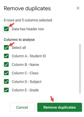
- Configure Settings:
- Check the option “Data has a header row” since your data includes headers.
- Make sure all columns are selected. You can manage column selection using the “Select All” checkbox.
- Remove Duplicates:
- Click the Remove duplicates button to initiate the process.
Example Scenario:
In your sample data, there are three records for the student Jesse Hill:
| 1001 | Jesse Hill | 10A | Maths | B |
| 1001 | Jesse Hill | 10A | Maths | B |
| 1001 | Jesse Hill | 10A | Science | B |
After duplicate removal, the records for Jesse Hill will be:
| 1001 | Jesse Hill | 10A | Maths | B |
| 1001 | Jesse Hill | 10A | Science | B |
This outcome occurs because the rows differ in the fourth column (Subject).
Note:
If you wish to remove duplicates regardless of the Subject column, you should uncheck the Subject column (column D) within the Remove Duplicates window.
In short, ensure that you only select the columns you want to analyze for duplicates in the Duplicate Removal window under the “Columns to analyze” label.
The Remove Duplicates tool only removes values in the duplicate rows and moves the rows up. It doesn’t delete any rows in your sheet.
Removing Duplicates Using Formulas
There are specifically two functions in Google Sheets that can remove duplicates: UNIQUE and SORTN. While most of you may be familiar with the UNIQUE function, SORTN might be less common in other spreadsheet applications. However, SORTN offers powerful duplicate removal capabilities with its tie-mode #2.
We’ll explore both methods, keeping in mind that UNIQUE is a single-purpose function known for its simplicity.
Handling Multiple Occurrences of Rows with UNIQUE
To remove duplicates in your student data across columns A to E in Sheet1, you can use the following formula:
=UNIQUE(Sheet1!A1:E)I suggest using this formula in a new sheet within the same file, for example, in cell A1 in Sheet2.
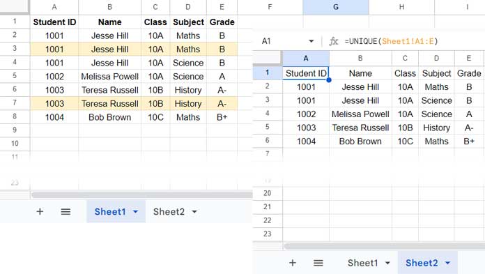
Similar to the built-in tool, it will remove duplicate records for Jesse Hill. Unlike the tool, you cannot specify to exclude the Subject column during formula execution.
In this context, the UNIQUE function simply removes multiple occurrences of rows based on all columns specified. It does not include a ‘Columns to analyze’ feature.
Handling Duplicates by Key Column Using SORTN
When using SORTN to remove duplicates, you should consider two key aspects:
- Exclude the header row when specifying the range and sort column ranges.
- Since SORTN is a sort function, the output will be sorted.
Similar to the built-in duplicate removal tool, to exclude the Subject column (D) while removing duplicates, you can use the following SORTN formula:
=SORTN(Sheet1!A2:E, 9^9, 2, Sheet1!A2:A&Sheet1!B2:B&Sheet1!C2:C&Sheet1!E2:E, 1)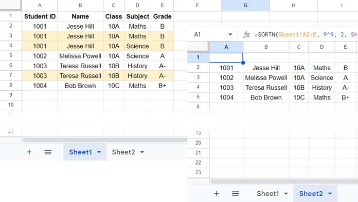
Let’s break down the formula. The syntax is:
SORTN(range, [n], [display_ties_mode], [sort_column], [is_ascending])Where:
range:A2:A(the data range excluding the header row)n:9^9(an arbitrarily large number specifies the maximum number of rows in the result)display_ties_mode:2(removes duplicate rows)sort_column:Sheet1!A2:A&Sheet1!B2:B&Sheet1!C2:C&Sheet1!E2:E(sorts and removes duplicates based on these columns, excluding column D)is_ascending:1(sorts in ascending order; specify0for descending order)
When applying this formula to a different dataset, you should only modify the range and sort_column parameters. The sort_column parameter acts as the key column, or what we can refer to as the ‘Columns to analyze’, for identifying and removing duplicates.
Removing Duplicate Rows Based on Minimum or Maximum Value
When using the built-in data removal tool or the SORTN function, which can analyze specific columns for duplicates, you might want to retain records with the minimum or maximum values.
To achieve this, you need to sort the data accordingly. For the Duplicate Removal tool, use the Data menu’s Sort range option to sort the data.
However, with SORTN, you can incorporate the SORT function within it. This poses a challenge because SORTN may not recognize ranges in the sort_column parameter.
Sample Data:
| Item | Vendor Name | Price |
| Laptop | ABC Electronics | 1000 |
| Laptop | XYZ Tech | 980 |
| Printer | XYZ Tech | 200 |
| Printer | ABC Electronics | 210 |
| Printer | PQR Inc. | 210 |
In this sample, column A (Item) is the ‘Column to analyze’ for duplicates. If you want to keep the least-priced items while removing duplicates, use the following solutions:
Using Duplicate Removal Tool:
- Select range A1:C and click Data > Sort range > Advanced range sorting options.
- Check “Data has header row”.
- Sort by Item (A to Z) and then Price (A to Z).
- Click Sort.
- Keep the data selected.
- Click on Data > Data cleanup > Remove duplicates.
- Check “Data has header row”.
- Uncheck all columns and check only “Item” under “Columns to analyze”.
- Click Remove duplicates.
This will give you the unique least-priced items.
| Item | Vendor Name | Price |
| Laptop | XYZ Tech | 980 |
| Printer | XYZ Tech | 200 |
Using SORTN:
=SORTN(SORT(Sheet1!A2:C, 1, 1, 3, 1), 9^9, 2, 1, 1)Here, the SORT function sorts the range A2:C (excluding the header row) based on column 1 (Item) in ascending order and then by column 3 (Price) in ascending order.
Syntax:
SORT(range, sort_column, is_ascending, [sort_column2, …], [is_ascending2, …])range:A2:Csort_column:1(Item)is_ascending:1(ascending order)sort_column2:3(Price)is_ascending2:1(ascending order)- The sorted result from SORT is then used as the range in SORTN.
In the SORTN sort_column parameter (Column to analyze for duplicates), instead of specifying A2:A (Item), we use column index 1. This is because the range is sorted, and specifying A2:A directly would reference the unsorted data.
What about Highest Priced Items?
To obtain the highest priced item:
- When using the Duplicate Removal tool, sort by Item in ascending order and Price in descending order.
- When using the SORT and SORTN combo, sort the data similarly within the SORT function.
Example using SORT and SORTN:
=SORTN(SORT(A2:C, 1, 1, 3, 0), 9^9, 2, 1, 1)Removing Duplicate Values Without Deleting Rows
If you want to remove duplicate values within rows without deleting the rows themselves in your source data, follow these steps:
Step-by-Step Instructions:
- Enter the Generic Formula:
Use the following generic formula to identify duplicate values within rows:
=ArrayFormula(COUNTIFS(ROW(first_column_range), "<="&ROW(first_column_range), columns_to_analyze, columns_to_analyze))Example Formula:
Assuming your student data is in A1:E where A1:E1 contains the header row, enter the formula in cell F2 (the column next to the last column and the row below the header row):
=ArrayFormula(COUNTIFS(ROW(A2:A), "<="&ROW(A2:A), A2:A&B2:B&C2:C&E2:E, A2:A&B2:B&C2:C&E2:E))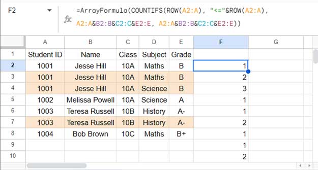
first_column_range:A2:A(the first column to analyze)columns_to_analyze:A2:A&B2:B&C2:C&E2:E(concatenated columns to analyze for duplicates)
This formula counts occurrences where concatenated values across columns A to E are duplicated within each row.
- Filter and Remove Duplicates:
- Select column F and click Data > Create a filter.
- Open the filter drop-down in cell F1, uncheck “1” (indicating non-duplicate rows), and click OK.
- Delete all visible values in columns A to E except the header row in the student data.
- Click Data > Remove filter to revert to the original view.
- Finally, remove the formula in cell F2.
This process effectively removes duplicate values within rows while preserving the row positions in your dataset.
Resources
- Compare All Columns with Each Other for Duplicates in Google Sheets
- Compare Two Tables and Remove Duplicates in Google Sheets
- How to Filter Duplicates in Google Sheets and Delete
- How to Filter Same-Day Duplicates in Google Sheets
- Remove Duplicate Values Within Each Row in Google Sheets
- How to Remove Duplicates from Comma-Delimited Strings in Google Sheets
- Find and Eliminate Duplicates Using Query Formula in Google Sheets


I’m not seeing where or how this is removing/deleting duplicates, I see it finds duplicates. But even using your sample pages I can’t get it to remove/delete duplicates.
What am I missing?
Thanks
Hi, Fred,
The formulas populate the data after eliminating/removing duplicates. You can see enough examples regarding this on this page.
If you want to permanently delete the duplicate content rows from the existing data range, follow this – How to Use Remove Duplicates Menu Command in Google Sheets.