With an advanced Array Formula, you can find multiple occurrences of Rows in Google Sheets. When I say multiple occurrences of rows, I mean the duplicate rows.

Other than the array formula, for those who like to have a more common formula, I have that solution too. I have a non-array COUNTIFS formula that finds the duplicate rows.

As you may already know, you need to copy and paste the non-array formula in each and every rows. But it has one advantage. You can use this formula in Conditional Formatting.

What are Multiple Occurrences of Rows and What We are Going to Do?

We are going to test whether the contents in selected columns in a row is not the second, third or any other occurrences in a range. In each and every row we will make this test.

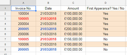
In this example the multiple occurrences are based on columns A and B. Here the Invoice Number 100005 in Cell A7 and its corresponding date in Cell B7 are the second occurrences of the values in row # 3, Cell A3 and B3. It’s the case with the values in row 5 and 9.

Wherever the second, third or any other occurrences occurred, the formula which we are going to discuss will return the value “No” in Column D, else “Yes”. The result “No” denotes the row is not the first appearance and it’s a duplicate row.

By testing so you are achieving the following goals.

1. Find duplicate rows based on single or multi-column matches. Wherever the formula puts “No”, that rows are duplicates. If the formula puts “Yes”, it’s called distinct rows.

2. Highlight Distinct rows/Multiple Nonoccurrence Rows or Multiple Occurrence Rows – Here I’ve highlighted the multiple nonoccurrence rows.

Here we begin.

The Step by Step Tutorial to Find Multiple Occurrences of Rows in Google Sheets

Here is the non-array formula to find and mark the second, third or any other occurrences of an item.

=IF(COUNTIFS($A$2:$A2, $A2, $B$2:$B2, $B2)=1, "Yes", "No")

You should key in this formula in Cell D2 and drag the fill handle to copy it to down until D9.

If you are not familiar in using Countifs formula in Google Sheets, here is a short description. But I suggest you check my Google Sheets Functions Guide to learn this function along with all other Count related functions.

Syntax:

COUNTIFS(criteria_range1, criterion1, [criteria_range2, criterion2, ...])

Actually, the Countifs formula counts the occurrences of items up to that row. For example, if you copy the above formula as said, the formula in cell E7 would be as below. Please use the Dollar symbols carefully.

=COUNTIFS($A$2:$A7, $A7, $B$2:$B7, $B7)

This Countifs formula counts the citeria_range1 A2: A7 and citeria_range2 B2: B7 for the match in criterion1 in A7 and criterion2 in B7.

Actually, this row # 7 is the second occurrences of the row # 3 in terms of values in column A and B. So the formula will return the number 2 as the result.

Wherever the value returned by Countifs is greater than 1, that means such rows are repeated ones or you can say duplicate ones. With Google Sheets IF logical test formula, you can return the value “No” in such rows. Here “No” means it is not the first appearances of that row.

Now you can automate this with an array formula. I’ll explain that later. Before that, you can see how to conditional format multiple occurrences of rows in Google Sheets. The same tips you can use to conditional format multiple nonoccurrences of rows.

How to Highlight Multiple Occurrences of Rows in Google Sheets

Highlighting multiple repeating rows in Google Sheets will be pretty easy if you have properly learned the above formula usage.

Select the range and apply the same above formula after removing the IF logical clause. But wait a moment. See the steps.

Steps:

Select the range A2: D12.

Go to Google Sheets Format Menu > Conditional Formatting.

In the Custom formula field, apply the below formula.

=COUNTIFS($A$2:$A2, $A2, $B$2:$B2, $B2)=1

Set the color and voila! You have set highlighting rules for the distinct rows. Change the last formula part form “=1” to “>1” to alter the coloring. This time it will highlight only the repeated rows.

As said above, we can find multiple occurrences of Rows in Google Sheets using an Array Formula too. Here is that awesome formula.

Array Formula to Find Multiple Occurrences of Rows in Google Sheets

First, let me provide you the formula. Here for clarification purpose, I am providing you the formula for single column match. Then I will tell you how to use this formula as above with two columns.

=ArrayFormula(IF(LEN(A2:A),if(
SORT(ROW(A2:A)-ROW(A2)+2,SORT(ROW(A2:A)-ROW(A2)+2,A2:A,1),1)-MATCH(A2:A,SORT(A2:A),0)=1,"Yes","No"),))

The SORT and MATCH functions are the basis of this Google Sheets formula to find and match multiple occurrences of items in Google Sheets.

This formula checks the invoice numbers in Column A and if it repeats in any rows, mark it with “No” saying it’s not the first appearance.

Note: You can skip this part if you feel it’s a little tough. To learn the usage of this formula in multiple columns, just jump to the end of this tutorial where you can see a screenshot. That reveals how to use this formula in two columns.

The Formula Logic:

First I am talking about thisSORT(ROW(A2:A)-ROW(A2)+2,A2:A,1) part of the formula.

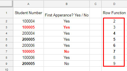
The Row function inside the formula will return the numbers from 2 to 9 as below.

Wherever you apply this formula, the numbering will start from two only and it’s a must. To do that, I’ve adjusted this Row Array formula accordingly.

Sort Formula Part:

The SORT formula sorts this row formula output based on the values in Column A (Student Number) in ascending order.

Syntax:

SORT(range, sort_column, is_ascending)

In our above Sort formula (under the formula logic), the sort range is the output of the above said row function. That’s the sequential numbers from 2 to 9.

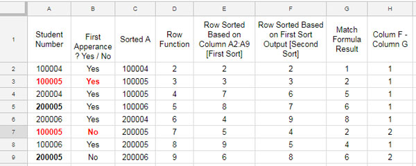
You can either use sort_column as a range or column number in the sort. Here I have used the student numbers in Column A as the sort column. To show you I have entered the result in Column E.

In Column C, I’ve just sorted Column A values (Student Number) for your reference and in Column D the sequential numbers.

Now when you check the above sort formula output in Column E, you can understand one thing. The numbers in Column E are arranged against its corresponding values in Column C. You can compare that with the Column A and D values.

Now the second sort formula also takes the same row numbers as sort range. But this time instead of Column A, the sorting is based on the value returned by the above mentioned Sort formula 1 (Column E). You can refer to Column F on the above screenshot to see the output.

It’s quite confusing, right? No need to hold a brainstorming session. In precise, you can read the above row, sort 1 and sort 2 formulas as below.

Generic Formula:

SORT(row numbers,SORT(row numbers,item in column A,1),1)

row numbers = sequential numbers from 2 to 9.

item in column A = student number in the range A2: A9

In short, the purpose of the above formula is a follows.

Suppose you have the above values in the range A2: A9 in a new tab. Sort that in ascending order. Now enter the numbers 2 to 9 in the range B2: B9 in that tab. Then drag and drop the rows to arrange as per our original data. See the sequential numbers. It would be placed as per the above formula output.

Match Formula Part:

In a sorted data you can use the below generic formula to find the occurrences of items.

sequential numbers (must start from 2) - relative position of items = group wise numbering.

The relative position we can find using the Match function.

Ours is an unsorted data. So we have sorted the sequential numbers as per the unsorted list.

The Match formula returns the relative position of items in Column A. Not the exact relative position but the relative position of the sorted items.

MATCH(A2:A,SORT(A2:A),0)

Syntax:

MATCH(search_key, range, [search_type])

Please refer the Match formula result in Column G on the screenshot above. In Column H, I’ve just deducted Column G value from Column F.

As you can see it returns 1 for the nonrepeated items. If the item repeats, you will get the count of that item in increment.

When you scroll back and check my final formula, you can see that I’ve used an IF Logical test to put “Yes” for the value 1 and if the value is more than one the formula will put “No”.

This formula returns the same result returned by our COUNTIFS formula. The difference, it’s an Array Formula and so no need to copy and paste in all rows.

Just like the Countifs non-array formula, you can use two columns in this array formula too. Please refer to this screenshot. I have marked where you want to make the changes.

In both Sort and Match formulas, replace the range A2: A with the underlined formula that uses CONCAT function.

Update: See the above image. There are actually three Concat formulas. By mistake, I only underlined two.

This combines Column A and B. If you want to check multiple occurrences in any other columns, you can change this part. That means you are not limited to use this formula in two columns. That’s all.

By using any of the above two formulas, you can find multiple occurrences of Rows in Google Sheets.

Additionally, you can use this formula for identifying duplicates. If you apply this formula to your sheet, you will understand this.