This tutorial covers an efficient solution to randomly select N numbers or values in Google Sheets. The key functions used are SORTN, UNIQUE, and RANDARRAY. If the list contains duplicates, the formula will automatically select only the unique values.

Real-Life Applications

Here are some scenarios where this formula can be applied:

• Selecting a random group of players.
• Choosing N winners in a lottery.
• Excluding excess participants randomly when you have a limited quota.

Formula to Randomly Select N Numbers

=LET(
  range, TOCOL(UNIQUE(cell_range), 3), 
  SORTN(range, n, 0, RANDARRAY(ROWS(range)), 1)
)

In this formula:

• Replace cell_range with the column reference containing the values you want to randomly select.
• Replace n with the number of random values you want to pick. If the cell_range contains fewer numbers than the value specified in n, the list will be returned as is, but without duplicates.

This formula works for randomly selecting numbers, text, or any other data types.

Example: Randomly Selecting N Values

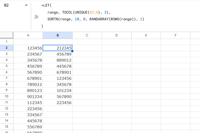
Suppose you have lottery serial numbers in the range A2:A and want to randomly pick 10 numbers without duplicates. Use the formula:

=LET(
   range, TOCOL(UNIQUE(A2:A), 3), 
   SORTN(range, 10, 0, RANDARRAY(ROWS(range)), 1)
)

Lottery numbers often include alphanumeric characters, such as AX-125467B. Since the formula works with any data type, it will efficiently pick N winners, regardless of whether the values are numeric or text.

Anatomy of the Formula

This formula has several components. Let’s break it down step-by-step. The LET function is used to simplify the formula by assigning names to intermediate results. Its syntax is:

LET(name1, value_expression1, [name2, value_expression2, …], formula_expression)

In the Formula:

• name1: range
• value_expression1: TOCOL(UNIQUE(A2:A), 3)

What Does value_expression1 Do?

• UNIQUE(A2:A): Extracts distinct values from the range. If the range contains empty cells, an empty string will appear in the result.
• TOCOL(..., 3): Converts the column into a single array while removing empty and error values.

This intermediate result (range) is then used in the next part of the formula.

The formula_expression Explained:

SORTN(range, 10, 0, RANDARRAY(ROWS(range)), 1)

Here’s how this works:

• SORTN: Selects and sorts the top N rows.
• range: The array of unique values generated earlier.
• n: 10, the number of random values to return.
• display_ties_mode: 0, ensures only the first 10 rows are returned.
• sort_column: RANDARRAY(ROWS(range)), generates random numbers for sorting.
• is_ascending: 1, sorts the random numbers in ascending order.

This ensures that 10 random values are selected and sorted.

Prevent the Formula from Changing on Every Update

By default, RANDARRAY is volatile, meaning the results refresh every time you edit the sheet or at specific intervals set under File > Settings. If you want the formula to remain static until triggered, you can use the LAMBDA function.

Steps:

1. Insert a tick box in an empty cell (e.g., B2) via Insert > Tick Box.
2. Use this modified formula in C2:

=IF(
   B2=FALSE, ,
   LAMBDA(
      randN, SORTN(TOCOL(UNIQUE(A2:A), 3), 10, 0, randN, 1)
   ) (RANDARRAY(ROWS(TOCOL(UNIQUE(A2:A), 3))))
)

Explanation:

• When B2 is unchecked (FALSE), the formula returns an empty string.
• When checked, it randomly selects N numbers/values.
• randN: A name assigned to RANDARRAY(ROWS(TOCOL(UNIQUE(A2:A), 3))) within the LAMBDA function.
• LAMBDA Syntax:

=LAMBDA([name, ...], formula_expression)(function_call, ...)

Here:

• name: randN
• formula_expression: SORTN(TOCOL(UNIQUE(A2:A), 3), 10, 0, randN, 1)
• function_call: RANDARRAY(ROWS(TOCOL(UNIQUE(A2:A), 3)))

This approach prevents the formula from recalculating unless you toggle the tick box.

Additional Resources

• Pick a Random Name from a Long List in Google Sheets
• How to Shuffle Rows Randomly in Google Sheets
• Google Sheets: Macro-Based Random Name Picker
• Randomly Extract a Percentage of Rows in Google Sheets
• Generate Odd or Even Random Numbers in Google Sheets
• Pick Random Values Based on Condition in Google Sheets
• Interactive Random Task Assigner in Google Sheets
• Generate Random Groups in Google Sheets