This guide will show you how to create a macro-based random name picker in Google Sheets, customized to fit your needs.
Before we jump in, here are some common questions you might have and their answers. These will help you determine whether this method suits your requirements.
Can I select multiple winners?
Absolutely! You can easily decide how many winners to pick—such as a first winner, second winner, and so on. With a small adjustment to the provided formula, you can select multiple winners effortlessly.
Can it handle a large number of participants?
Yes! This method works seamlessly, even with hundreds or thousands of participants. You can select winners randomly from a large dataset without any issues.
Can I use it for lotteries or other types of giveaways?
Yes, this method is highly versatile. Whether you’re selecting names, lottery numbers, or any other type of data, the same macro-based approach applies. Just ensure your data is prepared in the correct format, as explained in the guide.
Preparing the Data
Before recording the macro, organize your data in a structured format. For example:
- The first column should always contain unique IDs, manually entered (do not use formulas like SEQUENCE or ROW).
- If you only want to pick names, ensure column A contains IDs and column B contains names.
- In this example, we’ll randomly pick a winner along with their associated data. We’ll use the range
A2:Ffor selecting winners (with headers inA1:F1, which will be excluded).
| A | B | C | D | E | F |
| ID | First Name | Last Name | Phone | Time Stamp | |
| 1 | [email protected] | Lynn | Maxwell | 159487263 | 2018-04-18 10:15:07 |
| 2 | [email protected] | Daniel | Wheeler | 123456789 | 2018-04-18 08:15:46 |
| 3 | [email protected] | Rodney | Powell | 987654321 | 2018-04-19 08:48:12 |
| 4 | [email protected] | Allan | Washington | 456789123 | 2018-04-19 09:15:03 |
| 5 | [email protected] | Daisy | Evans | 369258147 | 2018-04-18 12:15:07 |
| 6 | [email protected] | Carla | Moore | 741852963 | 2018-04-18 12:18:07 |
Applying the Formula
To display random winners, enter the following QUERY formula in H2:
=QUERY(A2:F, "SELECT * WHERE A IS NOT NULL LIMIT n")- Replace
nwith the number of winners you want to pick. - Update
A2:Fto match the range of your data.
When you run the macro, it will randomize the range. The formula will then select the top n rows from the newly randomized range. This is the logic behind the macro-based random name picker.
Note: Ignore the current results in cell H2 until after running the macro, as they won’t reflect the randomized output yet.
Recording the Macro for Random Name Selection
Follow these steps to record the macro:
- Navigate to the first cell of your data (e.g., A2, below the header row).
- Click Extensions > Macros > Record Macro.
- Select the entire data range (e.g., A2:F). Use these shortcuts for quick selection:
- Windows: Press
Ctrl + Shift + Right(repeatedly if there are empty cells) and thenCtrl + Shift + Down(until the entire range is selected). - Mac: Use
Command + Shift + RightandCommand + Shift + Down.
- Windows: Press
- Click Data > Randomize Range.
- Click Save to stop recording the macro.
- Name the macro (e.g., “Winner”). Optionally, assign a shortcut like
Ctrl + Alt + Shift + [Number](orCommand + Option + Shift + [Number]on Mac). - Click Save.
Running the Macro
Running the macro to pick random names is straightforward:
Go to Extensions > Macros > Winner. If this is your first macro in the sheet, you’ll be prompted to authorize it. Follow the on-screen instructions to grant the necessary permissions.
The formula will then return the randomly selected winners.
Reverting the Randomization
If you wish to remove the randomization and restore the original order of the table:
- Sort the table by the first column (Serial Number/ID) in ascending order.
This will reset the data to its original order since we added serial numbers in the first column for this purpose.
Note: Once you reset the order, the randomization will be lost, and you’ll need to run the macro again to pick new random winners.
Additional Tip: Toggle Winners Display
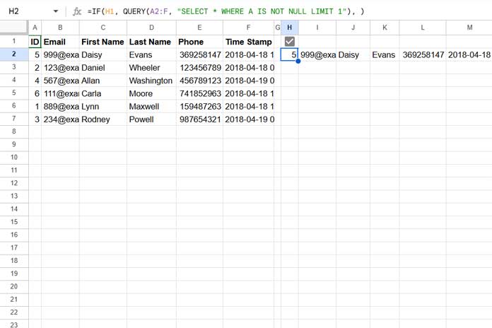
To hide or display the winners dynamically, use a checkbox:
- Navigate to H1 and insert a checkbox:
- Click Insert > Tick Box.
- Replace the formula in H2 with the following:
=IF(H1, QUERY(A2:F, "SELECT * WHERE A IS NOT NULL LIMIT n"), )When the checkbox is ticked, the winners will appear. When unticked, the cell will be blank.
Resources
- How to Record and Run Macros in Google Sheets
- Increase/Decrease Indent in Google Sheets [Macro]
- Pick a Random Name from a Long List in Google Sheets
- How to Shuffle Rows Randomly in Google Sheets
- How to Randomly Select N Numbers from a Column in Google Sheets
- How to Randomly Extract a Certain Percentage of the Rows in Google Sheets
- How to Generate Odd or Even Random Numbers in Google Sheets
- Pick Random Values Based on Condition in Google Sheets
- Interactive Random Task Assigner in Google Sheets
- How to Generate Random Groups in Google Sheets


