In Google Sheets, you can easily pick a random name from a long list using formulas or Apps Script. Whether you need a random student picker, giveaway winner selector, or team assignment tool, this tutorial explains both dynamic and static methods step by step.

It’s easy to pick a random name from a long list in Google Sheets using built-in formulas. However, while formulas are convenient, they can sometimes return different results every time the sheet recalculates because they use volatile functions.

In other words, whenever you edit the sheet or reload it, the randomly selected name may change. If you need a static (fixed) random result, Apps Script is a better solution.

Step-by-Step Instructions

Let’s assume you have a long list of student names in column A (A2:A) in Google Sheets, where A1 contains the header. Your goal is to pick a random name from the list.

Formula to Pick a Random Name in Google Sheets

You can use the following formula to select a random name from the range:

=SORTN(TOCOL(A2:A, 1), 1, 0, RANDARRAY(ROWS(TOCOL(A2:A, 1))), TRUE)

How This Formula Works

• TOCOL(A2:A, 1) → Removes empty cells from the list
• The second argument (1) tells SORTN to return only one random name
• The third argument (0) keeps the default duplicate handling behavior
• RANDARRAY(ROWS(TOCOL(A2:A, 1))) → Generates random numbers for sorting
• TRUE → Sorts in ascending order based on random values

In short:

SORTN sorts the list using randomly generated values and returns the first result.

To Get 5 Random Names

Simply change the second argument in SORTN:

=SORTN(TOCOL(A2:A, 1), 5, 0, RANDARRAY(ROWS(TOCOL(A2:A, 1))), TRUE)

Limitation of the Formula

The main issue with this approach is that it is volatile.

Since RANDARRAY is a volatile function, the selected random name changes whenever the spreadsheet recalculates, such as when:

• you edit a cell
• reload the sheet
• make structural changes to the spreadsheet

So, you will not get a fixed result.

Also, if your source list contains duplicate names, both the formula and script methods may return duplicates because each row is treated as a separate entry.

How to Keep the Random Name Static

If you want the selected random names to remain unchanged, you should use Apps Script.

This is especially useful when you want:

• a random student picker
• a winner selection tool
• a task assignment system

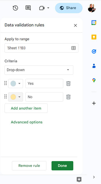
Step 1: Create a Drop-Down Control

To control when random selection happens:

1. Go to cell B3
2. Click Insert → Drop-down
3. Set options:
   • Yes
   • No
4. Click Done

Alternatively, you can use:

@ → Drop-downs → Yes/No

This will act as a trigger for generating random names.

Step 2: Add Apps Script

Go to:

Extensions → Apps Script

Replace the existing code with:

function onEdit(e) {
  const sheet = e.source.getActiveSheet();
  const range = e.range;

  const targetSheetName = "Sheet1";
  const dropdownCell = "B3";
  const outputStartCell = "C2";
  const numNamesToReturn = 1;

  if (sheet.getName() !== targetSheetName) return;
  if (range.getA1Notation() !== dropdownCell) return;

  const value = range.getValue();
  const outputCell = sheet.getRange(outputStartCell);
  const startRow = outputCell.getRow();
  const startCol = outputCell.getColumn();
  const lastRow = sheet.getLastRow();

  // Helper to safely clear old output down to the last data row
  const clearOldOutput = () => {
    if (lastRow >= startRow) {
      sheet.getRange(startRow, startCol, lastRow - startRow + 1, 1).clearContent();
    }
  };

  if (value !== "Yes") {
    clearOldOutput();
    return;
  }

  if (lastRow < 2) return;

  const names = sheet
    .getRange(2, 1, lastRow - 1, 1) // A2:A(lastRow)
    .getValues()
    .flat()
    .filter(v => v !== "");

  if (names.length === 0) return;

  // shuffle
  for (let i = names.length - 1; i > 0; i--) {
    const j = Math.floor(Math.random() * (i + 1));
    [names[i], names[j]] = [names[j], names[i]];
  }

  const selected = names
    .slice(0, numNamesToReturn)
    .map(v => [v]);

  // Clear ALL previous output data first so no leftovers remain
  clearOldOutput();

  // Write new values
  sheet.getRange(startRow, startCol, selected.length, 1).setValues(selected);
}

Step 3: Save the Project

Rename your project to something like:

randomname

Then click Save.

How the Script Works

The script runs automatically whenever cell B3 is edited.

• When the drop-down value is Yes, the script randomly selects names from column A
• The selected names are displayed in column C
• When the drop-down value is No, the output is cleared

To Get 5 Random Names Using Apps Script

Change:

const numNamesToReturn = 1;

to:

const numNamesToReturn = 5;

Sample Sheet

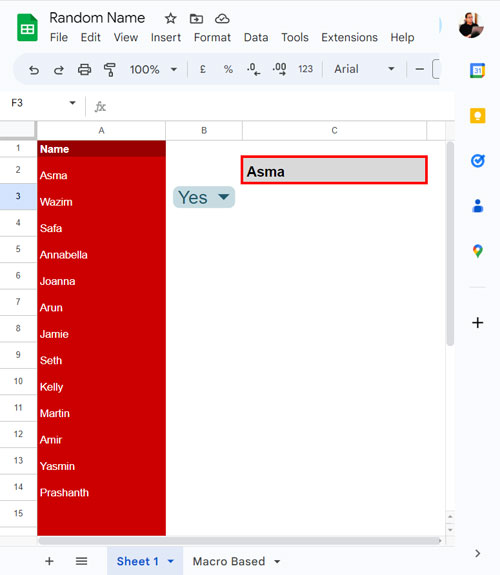
You can use the sample sheet with the script and drop-down already set up.

Simply replace the names in column A, then toggle the Yes/No drop-down in cell B3 to generate random selections.

Preview and Download

Conclusion

Using formulas is the quickest way to pick a random name in Google Sheets, but the results change whenever the sheet recalculates. If you need a fixed random selection, Apps Script provides a more reliable solution for student pickers, giveaways, and automated assignments.

Useful Resources

• Google Sheets: Macro-Based Random Name Picker
• How to Randomly Select N Numbers in Google Sheets
• How to Randomly Extract a Certain Percentage of the Rows in Google Sheets
• Pick Random Values with Conditions in Google Sheets
• How to Generate Random Groups in Google Sheets