In this tutorial, we’ll walk through the process of using macros to increase and decrease indentation in Google Sheets. While this method has its pros and cons, it provides a practical solution for formatting text with indentation without disrupting formulas.
Indentation is a common formatting style in word processing applications, such as Google Docs. Some spreadsheet applications, like Excel, also include this feature. In Excel, indentation is typically used to visually move text away from the left edge of a cell.
While you could manually add spaces by pressing the spacebar before entering text, this approach can create problems with functions like VLOOKUP, XLOOKUP, SUMIF, MATCH, and QUERY in Google Sheets. These formulas may fail to match indented text against criteria due to the added spaces.
Macro-based indentation in Google Sheets, however, avoids this issue. It does not introduce actual whitespace into a cell. Instead, it adjusts the appearance of the text while keeping its length unchanged. This ensures that formulas remain unaffected and function correctly.
In my Excel days, indentation was one of my favorite formatting tools. Unfortunately, Google Sheets does not natively offer this feature. However, by leveraging macros, you can replicate the functionality of increasing and decreasing indentation levels in Google Sheets.
I hope Google will eventually introduce dedicated “Increase Indent” and “Decrease Indent” buttons, similar to those in Excel, to make this process more straightforward.
Increase Indent Example in Google Sheets:
Decrease Indent Example in Google Sheets:
Pros and Cons of Macro-Based Indentation in Google Sheets
Using a macro, you can record UI interactions to simulate increasing or decreasing indentation in Google Sheets. Once recorded, you can run the macro from the Extensions menu or use an assigned keyboard shortcut, which starts with Ctrl+Alt+Shift. Like any macro, there are pros and cons to this method.
Pros:
- Easy to create and apply custom indentation in Google Sheets.
- Does not add any whitespace, so you can use functions like LEN or LEFT to verify the length of the indented text.
- Simple to apply indentation via the Extensions menu > Macros.
- You can also use keyboard shortcuts.
- It’s possible to format single cells, ranges, or even non-adjacent ranges with an Increase/Decrease indent.
Cons:
- Slower processing compared to using the normal menu or keyboard shortcuts.
- Only available within the spreadsheet where the macros are created (though there is a workaround below).
- The major limitation is that the macros are not available across all new files unless manually copied.
Workaround for Using Recorded Macros in All New Files
Here’s how you can make the indentation macros available in new Google Sheets files:
- First, set up the indentation macros in a new Google Sheets file and name it “Draft.”
- The next time you want to create a new file, open the “Draft” file, and go to File > Make a copy.
- In the copied file, add a new tab and delete the existing tab(s). The indentation macros will remain available in the new file.
How to Get Increase Indent in Google Sheets
To create indentation macros, we’ll record the necessary steps. I’ll demonstrate by recording four macros, each increasing the indentation by one space. These macros can also be used to decrease indentation by adjusting the space.
Let’s start with the first macro:
- Click on any blank cell or a cell containing text.
- Go to Extensions > Macros > Record macro.
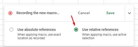
- Ensure that “Relative references” is selected (do not click Save or Cancel just yet).
- Navigate to Format > Number > Custom number formats.
- In the custom format field, press the spacebar once and type @.
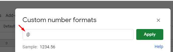
- Click Apply to save the new custom number format for indentation.
- Once the macro records the UI interaction, click Save.
- Name the macro “Indent 1” and assign it the shortcut Ctrl+Alt+Shift+1.
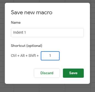
- Click Save.
We’ve now created a macro to indent text in Google Sheets.
Testing the Macro and Shortcut
To test the macro:
- Enter some text, such as “Info Inspired,” in a cell (e.g., B2).
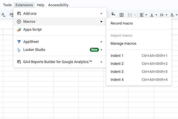
- Go to Extensions > Macros > Indent 1.
- Since this is your first time running the macro, you will need to authorize Sheets to run it. Follow the on-screen instructions.
After authorization, the macro will apply the increase indent to the text in the selected cell.
Adding More Indentation
Repeat the steps above to create additional indentation macros. Here’s how:
- Indent 2: Use two spaces before the @ symbol in the custom number format.
- Indent 3: Use three spaces before the @ symbol.
- Indent 4: Use four spaces before the @ symbol.
Make sure each macro is named appropriately and assigned a unique shortcut (e.g., Ctrl+Alt+Shift+2, Ctrl+Alt+Shift+3, etc.).
Testing Multiple Indentation Shortcuts in Google Sheets
To apply multiple indentations:
- Select a range of cells (e.g., A4:A6).
- Go to Extesnsions > Macros and select the desired indent level (e.g., “Indent 4”).
- The selected text will be indented according to the macro you applied.
If you want to indent text in two non-adjacent ranges (e.g., A4:A6 and A8:A10):
- Click on cell A4, hold Shift, and click on A6.
- Hold Ctrl and click on A8, then hold Ctrl+Shift and click on A10.
- Press Ctrl+Alt+Shift+4 or select ‘Indent 4’ from the Extensions menu to apply the indentation.
How to Decrease Indent in Google Sheets
To remove indentation, select the cells and go to Format > Number > Automatic.
To decrease indentation, apply a lower indent (e.g., Indent 1 or Indent 2) to the same cells.
Test Indented Text with LEN or LEFT
To verify that indentation doesn’t affect the length of the text, enter the text “Test” in cell A1 and use the following formula in cell B1:
=LEN(A1)This formula will return 4 (the length of “Test”). Now, apply Indent 2 (Ctrl+Alt+Shift+2) to cell A1. The LEN function will still return 4, confirming that indentation only affects the visual appearance and not the actual length of the text.
Number Formatting: Things to Remember
While the indent feature works with text and numbers, it’s important to note that it changes the number format to text. If you apply indentation to a cell containing a number, Google Sheets will treat it as text. For example, if you apply Indent 3 to cells A8:A10, containing numbers like 50, 100, and 150, a SUM formula will return 0.
To fix this, use the following formula:
=ArrayFormula(SUM(VALUE(A8:A10)))That’s it! You can now use macros to increase or decrease indentation in Google Sheets. Enjoy formatting your text without worrying about formula conflicts.
Resources
- How to Record and Run Macros in Google Sheets
- Google Sheets: Macro-Based Random Name Picker
- Inserting Bullet Points in Google Sheets
- 5-Star Rating in Google Sheets Including Half Stars
- Rate with Ease: Google Sheets’ New Built-In Rating Feature
- Insert Special Characters Without an Add-on in Google Sheets
- How to Insert Subscript and Superscript Numbers in Google Sheets


