There are four ways to insert bullet points in Google Sheets: using a keyboard shortcut, copy-pasting from other applications/web pages, custom number formatting, and using formulas.
I recommend using custom formatting for creating bullet lists in Google Sheets, as it doesn’t involve adding a physical character at the beginning of the list items.
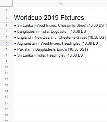
Example of a Bulleted List in Google Sheets:
Option 1: Adding Bullet Points Using a Keyboard Shortcut
This is the easiest way to add bullet points in Google Sheets. In this approach, you insert a bullet point before typing list items.
For example, assume you have the label “World Cup 2019 Fixtures” in cell A2 and the fixture “Sri Lanka v West Indies, Chester-le-Street (10:30 BST)” in cell A3.
Here is how to insert a bullet point before writing the list items:
- Double-click cell A3.
- Press
Alt + 7(Windows) orOption + 8(Mac). If it doesn’t work in Windows, try using the7key on the numeric keypad. - Press the space bar.
- Enter “Sri Lanka v West Indies, Chester-le-Street (10:30 BST).”
Follow the same process for cells A4, A5, and so on.
Option 2: Adding Bullet Points Using Copy-Paste
If you want different bullet styles, such as white bullets, inverse bullets, or circled bullets, the best option is to copy them from web pages or Google Docs and paste them into Google Sheets. Here’s how:
1. Copy and Paste Special Characters from Google Docs to Sheets
- In your browser’s address bar, type
https://docs.new/and press Enter to open a new Google Docs file. - Click Insert > Special characters.
- In the Special Characters window, type “bullet” in the search field.
- Click on the bullet point you want to insert into the document.
- Highlight the inserted bullet point, right-click, and select Copy.
- Double-click cell A3 in Google Sheets.
- Right-click and select Paste.
2. Copy and Paste Special Characters from This Page
You can copy the bullet points from the third column of the table below and paste them into your Google Sheets.
| Bullet Name | Formula | Symbol |
| Bullet | =CHAR(9679) | ● |
| White Bullet | =CHAR(9675) | ○ |
| Triangular Bullet | =CHAR(8227) | ‣ |
| Hyphen Bullet | =CHAR(8259) | ⁃ |
| Inverse Bullet | =CHAR(9688) | ◘ |
| Inverse White Bullet | =CHAR(9689) | ◙ |
| Circle White Bullet | =CHAR(9678) | ◎ |
| Circled Bullet | =CHAR(9673) | ◉ |
| Star Bullet | =CHAR(9733) | ★ |
| White Star Bullet | =CHAR(9734) | ☆ |
| Inverse Star Bullet | =CHAR(10026) | ✪ |
| Flower Symbol | =CHAR(10020) | ✤ |
| Sixteen Pointed Asterisk Symbol | =CHAR(10042) | ✺ |
| Snowflakes Symbol | =CHAR(10052) | ❄ |
| Rotated Heavy Black Heart Symbol | =CHAR(10085) | ❥ |
| Rotated Floral Heart Symbol | =CHAR(10087) | ❧ |
| Hand Symbols | =CHAR(9754) | ☚ |
=CHAR(9755) | ☛ | |
=CHAR(9756) | ☜ | |
=CHAR(9758) | ☞ |
Option 3: Adding Bullet Points Using a Formula
The table above contains different formulas based on the CHAR function. You can use one of them. Here’s an example:
To insert the Inverse Bullet symbol, use:
=CHAR(9688)Assume your list is in A3:A. Use the following array formula in cell B3:
=ArrayFormula(IF(LEN(A3:A), CHAR(9688) & " " & A3:A, ""))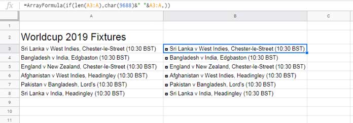
Converting Formula-Based Bullets to Static Text
- Highlight the range
B3:B8and copy the content. - Right-click cell
A3, then select Paste special > Paste values only. - Delete the formula in cell
B3.
Option 4: Custom Formatting for Bullet Lists in Google Sheets
I have already explained how to insert bullet symbols using the CHAR function. You can also use this method to create a formatted bulleted list.
For example, to use the Flower Symbol (✤) as a bullet:
Steps:
- Get the Symbol in a Blank Cell
- Enter
=CHAR(10020)in any blank cell (e.g., G1). - Copy the content using
Ctrl + Cor right-click and select Copy.
- Enter
- Select the Cell to Apply the Bullet
- Navigate to cell C3 (where you want to apply the Flower bullet).
- Apply Custom Formatting
- Go to Format > Number > Custom Number Format.
- In the blank field, paste the Flower symbol (
Ctrl + Vor right-click and select Paste). - Tap the space bar and type
@, then click Apply. For more spacing, press the space bar multiple times.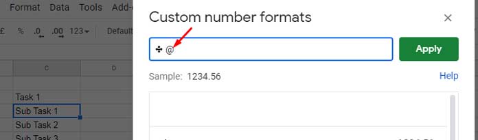
- Apply Formatting to Other Cells
- Copy the formatted cell (C3), select the range
C4:C6, right-click, and choose Paste special > Paste format only. - Repeat this for
C8:C11, or use the Format Painter.
- Copy the formatted cell (C3), select the range
This method allows you to create a bullet list in Google Sheets without adding physical characters.
Which Method Should I Choose?
- Keyboard shortcut: The easiest option for quick bullet insertion.
- Copy-pasting: Ideal if you need custom bullet styles.
- Formula-based approach: Useful if you want dynamically generated bullets.
- Custom formatting: Best if you don’t want a physical character affecting formulas or lookups.
That’s all! I hope you found these tips on inserting bullet points in Google Sheets helpful.
Related Resources
- Rate with Ease: Google Sheets’ New Built-In Rating Feature
- How to Create First Line Indent and Hanging Indent in Google Docs
- Increase and Decrease Indent in Google Sheets with Macro
- Formula-Based Conditional Indentation in Google Sheets
- Restrict Entering Special Characters in Google Sheets (Data Validation)
- Highlight Cells Containing Special Characters in Google Sheets
- Insert Special Characters Without an Add-on in Google Sheets
- 5-Star Rating in Google Sheets Including Half Stars


