I have the ratings of several products in a column, represented by numbers such as 1, 2, 3, 4, 5, 3.5, 4.5, etc. I want to create an in-cell 5-star rating system in Google Sheets that can represent these rating numbers (scores).
Assuming I have the number 4.5 in cell B2, I want to display a 4.5-star rating across the row C2:G2. In cells C2, D2, E2, and F2, there should be full stars (4 ratings), and in cell G2, a half-filled star should represent a 0.5 rating.
A single formula in cell C2 should generate the 5-star rating as described. The image below provides a visual representation of the in-cell 5-star rating in Google Sheets.
Two Methods for Creating a 5-Star Rating System in Sheets
There are two methods:
- Using in-cell images and an array formula.
- Repeating star character symbols (both white and black) using the REPT + CHAR combination formula.
Star Rating with In-Cell Images (Handles Half Stars)
A star rating that includes half stars is only achievable using the first method, which is the in-cell images.
Without a doubt, to create the 5-star rating system in Sheets as shown in the GIF above, I have utilized three-star images: a black star, a white star, and a half-filled star.
I will explain in a later part of this tutorial how to obtain free full and half-filled star images for use in Google Sheets to create the 5-star rating chart.
This will be discussed in detail in a separate section below.
Star Rating with REPT + CHAR Formula Method (No Half Stars)
The traditional method for creating a star rating table in Google Sheets involves using the CHAR (character) output from the REPT function, as shown below:
=REPT(CHAR(9733), 2)The formula above will repeat the black star symbol twice. To display a white star, change the number to 9734.
However, it’s important to note that this method doesn’t allow for half-star ratings because there is no representation of a half-filled star in the current Unicode table.
If you are adamant about using a character for a half-star, you can consider using the =CHAR(10028) formula, which is close to a half-filled star. Please be aware that this character is not a left-half black star, so it may not be a perfect match for your needs.
In reality, using the CHAR function in Google Sheets doesn’t provide a straightforward way to display a half-star, as there is no corresponding Unicode character for it.
Example:
Let’s use the character codes to create a 5-star rating system in Google Sheets:
I’ve book titles in B3:B6 and their numerical rating in C3:C6. Use the following formula in cell D3 to generate the star rating.
=ArrayFormula(IFERROR(REPT(CHAR(9733), ROUND(C3:C6))&REPT(CHAR(9734), 5-ROUND(C3:C6))))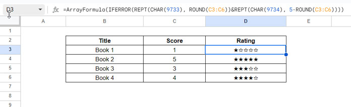
Formula Explanation
REPT(CHAR(9733), ROUND(C3:C6)): It repeats the black star symbol (★) a number of times equal to the rounded value of the numbers in cells C3:C6. For example, if a number in one of those cells is 4.2, it will round it to 4 and display four black stars.REPT(CHAR(9734), 5-ROUND(C3:C6)): This part repeats the white star symbol (☆) for the remaining positions to reach a total of 5 stars.
The & is used for concatenating the results.
The formula could return an error if the number is not between 0 and 5, including both values. The IFERROR function is used to prevent that error.
The ARRAYFORMULA signifies that the formula operates on an array of values (C3:C6), not just a single cell (C3).
Step-by-Step Guide to Creating an Image-Based 5-Star Rating in Sheets
As mentioned earlier, I’m going to use three images for our rating table. To get started, you’ll need those images, correct?
You can obtain it from the sample sheet provided below.
Get White, Black, Half Star Images
Full and Half-Filled Star Images in Sheets
I’ve already shared my sample sheet containing the images and my 5-star rating formula.
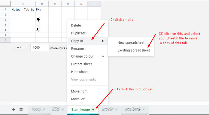
Open the sheet and right-click on the tab named “Star_Image.”
Select Copy to > Existing spreadsheet and choose the file in which you want to create the rating chart. Click “Insert.” For a clearer understanding, please refer to the instructions in the following image.
If you prefer, you can easily create a star image using the Photoshop Polygon tool. I won’t go into that here, as you can find several tutorials online. Additionally, I’ve already provided you with the necessary images above.
Note: After you copy the sheet, please rename it to ‘Star_Image.’ By default, it will be named ‘Copy of Star_Image.’
Data Preparation for Rating and Weighted Average
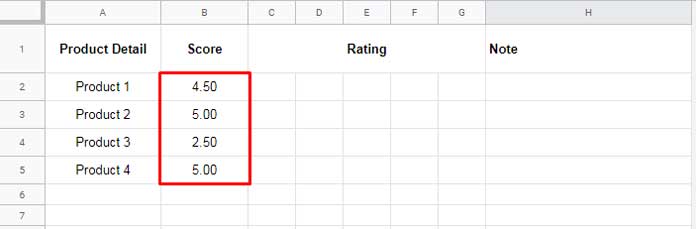
As you can see, I have already calculated the ratings in the background and filled them in column B. You might already have a system in place to determine the product rating on a scale from 1 to 5. You can match that rating with the respective product name.
If you are unsure about how to calculate the rating from user votes for each product, the following example will provide you with insight.
Let’s assume you’ve received user votes for product 1 as follows:
| Rating (1-5 stars) | User Votes |
| 1 star | 0 |
| 2 stars | 3 |
| 3 stars | 6 |
| 4 stars | 21 |
| 5 stars | 9 |
This means that 3 persons gave 2 ratings, 6 persons gave 3 ratings, and so on. By using the AVERAGE.WEIGHTED function, you can determine the overall rating of this product.
If the ratings are located under the label “Rating (1-5)” in the range A2:A6 (without the text star/stars) and the user votes are in B2:B6, you can use the following formula to calculate the weighted average. The formula will return 3.92, which means a rating of 3.92 out of 5 stars.
=AVERAGE.WEIGHTED(A2:A6, B2:B6)You can round this rating using the CEILING or FLOOR function as follows:
=CEILING(AVERAGE.WEIGHTED(A2:A6, B2:B6), 0.5)Result: 4 stars out of 5.
=FLOOR(AVERAGE.WEIGHTED(A2:A6, B2:B6), 0.5)Result: 3.5 stars out of 5.
The Formula to Create an In-Cell 5-Star Rating System in Sheets
Finally, I hope you are now ready to use the formula.
For my sample data provided above (please refer to the image below the subtitle ‘Data Preparation for Rating and Weighted Average’), you simply need to enter this formula in cell C2, and it will automatically expand to the rows and columns:
=ArrayFormula(IF(B2:B5<SEQUENCE(1, 5)-0.5, Star_Image!B4, IF(B2:B5<SEQUENCE(1, 5), Star_Image!B5, Star_Image!B3)))This formula is designed to create an in-cell 5-star rating system in Google Sheets based on the values in cells B2 to B5. Here’s an explanation of the formula:
IF(B2:B5<SEQUENCE(1, 5)-0.5, Star_Image!B4, …): This part of the formula checks if the values in cells B2 to B5 are less than a sequence of numbers from 0.5 to 4.5 and displays an empty star wherever the evaluation returns TRUE. For example, if the rating is 1.5, it will return TRUE in the last three cells.IF(B2:B5<SEQUENCE(1, 5), Star_Image!B5, …): This part of the formula checks if the values in cells B2 to B5 are less than a sequence of numbers from 1 to 5 and displays a half-filled star wherever the evaluation returns TRUE. For instance, if the rating is 1.5, it will return TRUE in the second cell.
The formula automatically fills the remaining cells with full stars.
That’s all. Enjoy!
Related: Rate with Ease: Google Sheets’ New Built-In Rating Feature


