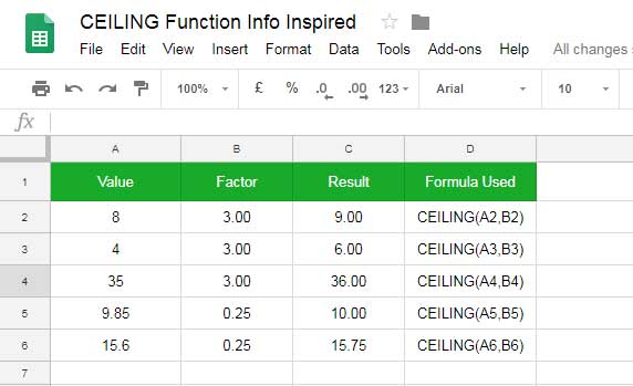
In one of my recent tutorial related to rounding of time, I have used the functions CEILING, FLOOR, and MROUND. Unfortunately that time I haven’t an individual tutorial for CEILING. To fill that, I’ve come up with this tutorial on the use of CEILING function in Google Sheets.
You can use the function CEILING in Google Sheets to round a number up to the nearest integer multiple of specified significance. Similarly to round a number down, the suitable function is FLOOR and just to round a number to the nearest integer multiple of another number you can depend on MROUND.
All these three functions are similar in use. So learning any one of them will make the learning of the other two functions easy.
Syntax:
CEILING(value, [factor])
Unlike MROUND and FLOOR, this time I’m taking you directly to the examples. The above arguments in the syntax are the same in FLOOR function. So if you want more details (not necessary for learning the Ceiling function), please refer my tutorial on the use of FLOOR function.
Example of the Use of CEILING Function in Google Sheets
Please go through the following Ceiling formulas. Do note that the formula results (Column C) would always be higher than or equal to the values (column A).

As an example, I am taking one formula from the above. Instead of cell references, I am entering the arguments within the formula.
=CEILING(8,3)
Result: 9
This formula is equal to the formula in cell C2. In this formula 8 is the “value” and 3 is the “factor”.
If you use the Floor function here, the result would be 6 as it rounds down to the nearest integer multiple of the factor. Here the Ceiling formula is rounding up like;
1 * 3 = 3

2 * 3 = 6

3 * 3 = 9
In this multiplication, the last part is the integer multiplication of factor 3. Here the value to rounds up is 8. So the formula returns 9 as it’s the rounded up value.
Note:
In the Ceiling formula, the argument “factor” is optional. You can’t use 0 as a factor. If you omit factor, it’ll be treated as 1 which is the default.
The Factor must be positive. But Value can be positive or negative.
The most common use of the function CEILING is to round up decimal places. To understand this, you can refer to the above example formula in Cell C6.
You can use the Ceiling function in Google Sheets to round up the denomination of currency.
For example, at the time of writing this post the exchange rate of INR to USD is 0.005, i.e., 1 INR is equal to 0.005 USD. So if you convert 1560.00 INR to USD, the amount would be 23.91 USD. Here you can use Ceiling formula as below.
=ceiling(23.91,0.05)
Result: 23.95
Similar: How to Convert Currency in Google Sheets
That’s all. Enjoy!


