Google Sheets now offers a new built-in rating feature that is significantly more convenient and dynamic than the CHAR method.
Over the years, we’ve been using combinations of CHAR and REPT or star images for a rating system in Google Sheets. However, you are no longer required to use them, even though they will still work.
Let’s explore this new feature with the examples below.
Google Sheets’ New Rating Feature Makes Star Rating a Breeze
The new built-in rating feature in Google Sheets is, in fact, a smart chip.
But what, precisely, is a smart chip?
Smart chips in Google Sheets are interactive elements that you can embed within cells in your spreadsheets. They enable you to include contextual information, such as locations, addresses, files, ratings, and more. Smart chips empower users to access relevant and accurate data directly within the spreadsheet environment.
Smart chips prove especially valuable for collaborative documents where multiple individuals are working on the same spreadsheet.
The new rating smart chip facilitates the inclusion of ratings into spreadsheet cells.
You can access this feature in two ways:
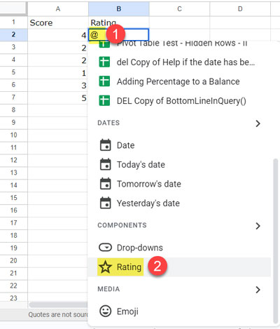
- Using the @-menu: Simply type @ in a cell, and a menu will appear.
- By clicking ‘Insert’ > ‘Smart chips’ > ‘Rating’.
Various Ways to Utilize the New Built-in Rating Feature in Google Sheets
Actually, the new built-in rating feature in Google Sheets is highly dynamic and versatile, allowing you to use it in various ways.
Conventional Way: Scores in One Column and Star Ratings in Another Column
In the conventional approach, you may have scores in one column and ratings in another column. For example, you have scores such as 4, 2, 2, 1, 3, and 5 in cells A2 to A7. You can apply the rating in cells B2 to B7 in different ways:
Type “@” in cell B2, scroll down, and click on “Rating,” or in cell B2, click on “Insert” > “Smart Chip” > “Rating.”
Then, in cell B2, enter the formula =A2 and press Enter.
Copy and paste the star rating from cell B2 to the cells in the range B3 to B7. Alternatively, you can drag the fill handle down in cell B2.
The feature is dynamic, so when you modify the scores in cells A2 to A7, the star ratings will update accordingly.
Format the Numbers to Star Rating
This is the easiest way to implement a star rating in Google Sheets. You can select the scores and apply the rating to them.
- Select the scores in A2:A7
- Click on “Insert” > “Smart Chips” > “Rating.”
Star Rating for Multiple People Working on the Spreadsheet
As far as I know, this is the primary reason for implementing the new built-in rating feature in Google Sheets. Here’s how it works:
Imagine you want to collect user feedback for an item in cell A2. Ask users to leave their ratings in cells B2 to E2. You can insert 0 rating stars in cells B2 to E2 by typing “@” and selecting “Rating.”
When a user clicks on the rating, a pop-up will appear with different rating options, and they can pick the one they prefer.
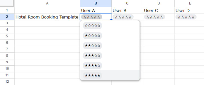
Alternatively, they can directly enter their score from 0 to 5, which will be converted to a star rating.
Other Advantages of Using the New Built-In Rating Feature in Google Sheets
The new built-in star rating feature has a few more additional advantages compared to the conventional star rating system in Google Sheets. Here are two of them.
- Highlighting: Since it maintains a numeric underlying value, you can utilize it for conditional formatting. You can adjust the rating color to green if it exceeds a particular value and to red if it falls below that value.
- Calculating Average Ratings: You can easily calculate the average rating from multiple-star ratings within a specified range.
For instance, the following AVERAGE formula returns the average of the ratings in the range B2 to E2:
=AVERAGE(B2:E2)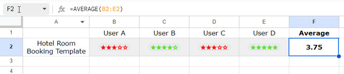
To implement the highlighting, you can create two conditional formatting rules within “Format” > “Conditional formatting” > “Custom formula is” for the apply-to range B2:E2:
Green:
=B2>3Set the fill color Green.
Red:
=B2<4Set the fill color to Red.
The first custom formula rule will highlight the star rating to green if the rating is greater than 3 (>3), and the second rule highlights the star rating to red if the rating is less than 4 (<4)
These rules will help you visually represent the ratings based on the specified conditions.


