Highlighting the Nth occurrence—such as the 2nd, 3rd, or 10th time a value appears—is very useful in Google Sheets. You might find this helpful in many real-life scenarios. For example:
- In a customer support log, you may want to highlight the third time a customer reports an issue—a sign that something’s not resolved. This helps escalate recurring problems and prioritize follow-ups.
- In a sales record, highlight the 10th purchase by a customer to trigger a loyalty reward or discount. It helps automate milestone tracking and improve customer retention.
- In offices, schools, or banks, highlight the second Saturday of a given month to identify a recurring holiday.
This tutorial shows you how to highlight the Nth occurrence in Google Sheets using conditional formatting—whether your data is arranged in columns or rows.
Highlight a Value’s 2nd, 3rd, or Nth Occurrence in a Column
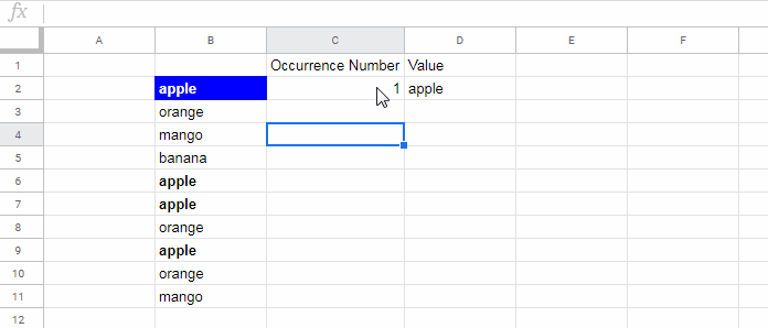
Let’s say you have a list of fruits in B2:B. You want to highlight, for example, the 3rd time a specific fruit appears.
Steps:
- Specify the occurrence number in cell
C2(e.g., 3). - Enter the value to highlight in cell
D2(e.g., “Apple”). - Select the range
B2:B. - Go to Format > Conditional formatting.
- Under Format rules, choose Custom formula is.
- Enter this formula:
=AND($B2=$D$2, COUNTIF($B$2:B2, $D$2)=$C$2) - Pick a formatting style and click Done.
This will highlight the Nth occurrence (as specified in C2) of the value you entered in D2.
How the Formula Works
The formula uses a running count:
COUNTIF($B$2:B2, $D$2)This counts how many times the value in D2 has appeared up to the current cell. If that count matches the number in C2, and the value matches D2, the cell gets highlighted.
Want to highlight the entire row instead of just the column? Just change the “Apply to range” in the sidebar to include full rows (like A2:D100).
Highlight a Value’s 2nd, 3rd, or Nth Occurrence in a Row
Most data is arranged in columns, but sometimes you might have values laid out across a row.
For example, let’s say the list is in row 2, from B2:Z2. You want to highlight the Nth occurrence of a specific item in that row.
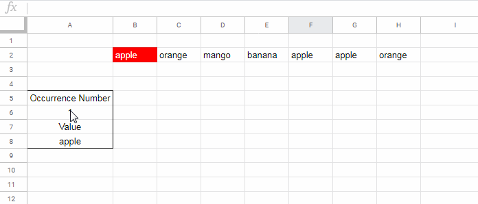
- Specify the occurrence number in cell
A6. - Enter the item to highlight in cell
A8.
Apply This Rule:
- Select the range
B2:Z2. - Use this conditional formatting formula:
=AND(B$2=$A$8, COUNTIF($B$2:B2, $A$8)=$A$6)
That’s how you can highlight the Nth occurrence in a row in Google Sheets.
If you want to highlight the entire column where that Nth occurrence appears (rather than just the cell in row 2), update the Apply to range in the sidebar to include all rows in those columns. For example:
Apply to range: B2:Z100
Keep the formula the same. Since the formula checks only row 2, but you’re applying formatting to full columns, only the column that contains the Nth match will be highlighted—across all rows in that column.
Final Thoughts
The ability to highlight the Nth occurrence in Google Sheets is incredibly helpful for tracking milestones, identifying repeat events, and triggering alerts or formatting based on patterns in your data.
To learn more ways to apply conditional formatting across different scenarios, including advanced use cases, explore the Ultimate Guide to Conditional Formatting in Google Sheets, where all tutorials are neatly organized.


Thank you, but what if I only want to highlight (or color) the nth occurrence of all cells in a column without precising one?
for example, when i put a condition like this :
=countif(B:B,B2)>1it gives all duplicates.
Hi, Jinane karhani,
This may help – Highlight Duplicates in Single, Multiple Columns, All Cells in Google Sheets.