This post shows how to select the required column from an array result in Google Sheets using simple formulas — no scripts or add-ons needed.
When a formula returns multiple columns, you might want to extract a specific column — whether it’s the first, middle, or last — based on your needs.
So, how do you select only the required column or columns from an array result in Google Sheets?
You can use four different functions in Google Sheets to accomplish this:
CHOOSECOLSINDEXARRAY_CONSTRAINQUERY
You might wonder: Why not use the OFFSET function? The reason is simple — OFFSET requires a reference to a physical cell range, not a virtual array generated by a formula. In other words, it doesn’t work well with dynamic array outputs (like those returned by FILTER, QUERY, etc.).
Ref.: Google Sheets function guide
Sample Data
Here’s the sample data (range A1:D9) for our demonstration:
| Name | Score 1 | Score 2 | Score 3 |
|---|---|---|---|
| Evan | 110 | 111 | 100 |
| Flora | 100 | 100 | 120 |
| Ben | 98 | 101 | 110 |
| Evan | 116 | 115 | 120 |
| Evan | 101 | 109 | 100 |
| Evan | 100 | 98 | 115 |
| Ben | 125 | 125 | 101 |
| Ben | 97 | 102 | 111 |
The following formula in cell F1 filters rows containing the name “Evan” and includes the header row:
={A1:D1; FILTER(A2:D9, A2:A9="Evan")}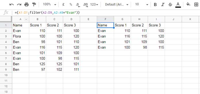
Select the Required Column in Google Sheets
Let’s now look at how to select only the required column from an array result in Google Sheets using each of the four mentioned functions — along with their pros and cons.
1. Select Required Columns Using CHOOSECOLS
This is the most straightforward function dedicated to selecting columns from an array result.
=CHOOSECOLS({A1:D1; FILTER(A2:D9, A2:A9="Evan")}, 1)Returns only the first column.
=CHOOSECOLS({A1:D1; FILTER(A2:D9, A2:A9="Evan")}, 1, 4)Returns the first and last columns.
Pros:
- Easy to use.
- Can select any column(s), in any order.
Cons:
- You can’t specify a range like “from column 2 to 4” directly — you’ll need to list out each column number or use
SEQUENCEto generate them dynamically.
2. Select a Column Using the INDEX Function
If you only need to extract a single column from an array, INDEX is a great choice.
=INDEX({A1:D1; FILTER(A2:D9, A2:A9="Evan")}, 0, 3)Returns the third column.
Pros:
- Shortest and simplest way to select an individual column from an array result.
- Eliminates the need to use
ARRAYFORMULA—INDEXhandles array expansion on its own.
Cons:
- Can return only one column at a time.
- For multiple columns, you’ll need to nest multiple
INDEXformulas — not ideal.
Example of combining multiple INDEX formulas:
={
  INDEX({A1:D1; FILTER(A2:D9, A2:A9="Evan")}, 0, 1),
  INDEX({A1:D1; FILTER(A2:D9, A2:A9="Evan")}, 0, 3)
}
3. Limit Columns Using the ARRAY_CONSTRAIN Function
If you want to select columns from the start of an array result, use ARRAY_CONSTRAIN.
=ARRAY_CONSTRAIN({A1:D1; FILTER(A2:D9, A2:A9="Evan")}, 9^9, 2)Returns the first two columns. The 9^9 represents a very large number, ensuring all rows are included.
Pros:
- Efficient and concise for selecting a set number of columns from the beginning.
- Performs well, especially compared to more complex formulas.
Cons:
- Only selects columns from the start of the array — you can’t pick random columns.
4. Select Required Columns Using the QUERY Function
Much like CHOOSECOLS, QUERY can pick any columns from the array, regardless of position.
=QUERY({A1:D1; FILTER(A2:D9, A2:A9="Evan")}, "SELECT Col1, Col4")Returns the first and fourth columns.
Pros:
- Flexible: pick any columns you want in any order.
Cons:
- Uses Google’s Visualization API Query Language — which may affect performance in very large sheets.
- You can’t specify a column range like “from column 2 to 4” directly — you need to list each column explicitly.
Bonus Tip: Search and Select a Column by Name
All the above methods require specifying the column number(s). But what if you want to search and select a column by its header name?
Here’s how you can use FILTER to select a column by name (e.g., “Score 2”):
=FILTER(A1:D9, A1:D1="Score 2")If you want to select multiple columns by name, you can combine XMATCH with FILTER:
=FILTER(A1:D9, XMATCH(A1:D1, {"Name", "Score 2"}))Simple and super useful when you don’t know the exact column positions!
Conclusion
To wrap up, if you’re dealing with dynamic arrays in Google Sheets, you can select only the required column from an array result using one of the following:
- Use
CHOOSECOLSfor flexibility. - Use
INDEXfor simplicity when picking a single column. - Use
ARRAY_CONSTRAINwhen working with a fixed number of leading columns. - Use
QUERYwhen selecting multiple arbitrary columns. - And finally, use
FILTERif you want to match a column by its header name.
You can swap the FILTER expression in any of these examples with another array-returning formula like GOOGLEFINANCE, SORT, or QUERY.
Related Tutorials
- Extract Last Value from Each Column in Google Sheets
- How to Sum Every Nth Row or Column in Google Sheets
- Get the Last Column from a Data Range in Google Sheets
- Dynamically Remove Last Empty Rows and Columns in Sheets
- Get the First or Last Row/Column in a New Google Sheets Table
- Dynamic Column References in Google Sheets Query
- Select Every Nth Column in Google Sheets Query – Dynamic Formula


Prashanth, do you know how to achieve the reverse of this? I want to retrieve the column index number of an array that can be used in a formula.
For instance, I need a formula that functions somewhat like this pseudocode:
=ArrayFormula(IF(OR(column_of_array=1, column_of_array=3), "do the thing", array)).In my specific case, I always have a 5-column array. If that information helps with suggesting a different solution, I’d appreciate it.
Thanks!
Hi McKay Savage,
You can utilize the LET function for this purpose:
=LET(name, your_formula, IF(OR(COLUMNS(name)=1, COLUMNS(name)=3), "do this", name))Simply replace your_formula with the specific formula you are working with.