You can utilize a BYCOL and XLOOKUP combo formula to extract the last values from each column in Google Sheets.

Firstly, I’ll provide you with the XLOOKUP formula to retrieve the last non-blank cell value from a single column. For this example, we will use column B. The value can be any type: number, date, string, timestamp, or special characters.

In the final section of this tutorial, we will narrow down the focus to extracting either numbers or strings from a mixed data type column range.

The following XLOOKUP formula will return the last non-blank value in column B:

=ArrayFormula(XLOOKUP(TRUE, B:B<>"", B:B, ,0,-1))

Here’s the breakdown:

• TRUE serves as the search key.
• B:B<>"" is the lookup range, and B:B is the result range.

Explanation:

• B:B<>"" returns TRUE (with ArrayFormula support) in non-blank cells and FALSE in blank cells. This is why we use TRUE as the search key.
• The formula performs an exact match of the search key (0 represents an exact match), and the search mode is -1, indicating the search is from the last value to the first value. This ensures that the formula finds and returns the last non-blank value in column B.

You can apply this formula to a specific range in a column as well. For instance, replace B:B with B10:B100.

Array Formula to Extract the Last Values from Each Column in Google Sheets

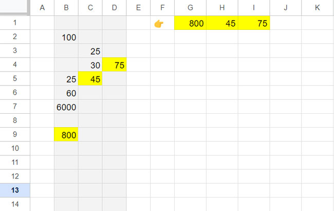
Now, to extract the last non-blank cell value in multiple columns, let’s consider an example where the range spans columns B to D, and the above formula is in cell G1.

To extend the formula manually, either drag the fill handle (the pointer at the bottom right corner of cell G1, when the current cell is G1) to I1, or select G1:I1 and use the shortcut keys Ctrl + R (Windows) or ⌘ + R (Mac).

If you want the formula to expand across and return the last non-blank cell value in each column within the specified range, use the BYCOL lambda function in conjunction with XLOOKUP.

Formula:

=BYCOL(B:D, LAMBDA(c, ArrayFormula(XLOOKUP(TRUE, c<>"", c, , 0, -1))))

Enter this formula in cell G1, and it will automatically expand to I1, assuming H1 and I1 are left blank to accommodate the expansion.

Sample Sheet

Formula Explanation

This formula follows the syntax:

BYCOL(array_or_range, LAMBDA([name, …], formula_expression))

• array_or_range: B:D – the range to find the last values from each column.
• name: c – represents the current column.
• formula_expression: ArrayFormula(XLOOKUP(TRUE, c<>"", c, ,0,-1)) – this is our XLOOKUP formula used to extract the last non-blank cell value in a column. The distinction here is the replacement of B:B with ‘c’.

The BYCOL function iterates over each column in the range, so ‘c’ in the lookup and result range becomes B:B, C:C, and D:D in each iteration.

This approach allows us to extract the last value from each column within a specified range in Google Sheets.

Extracting the Last Numbers or Strings from Each Column in a Range with Mixed Data Types

Can we specify extracting the last number or text string instead of ‘value’?

The above formula extracts the last non-blank cell value from each column irrespective of data type. The last value can be a number or string. Please note that dates and times are considered numbers in Google Sheets.

Here are the required changes to be specific to a number (including dates, timestamp, time) or string:

• To extract the last non-blank strings from each column in the range, replace c<>"" with ISTEXT(c).
• To extract the last non-blank numbers/dates/time/timestamp from each column in the range, replace c<>"" with ISNUMBER(c).

Resources

Finding the last value from each column has many real-life uses in Google Sheets. Assume you have a sequential date column A and category columns B, C, and D, where B1:D1 contains category names.

You can use the above formula to find the last value in each category column. You might want to use B2:D as the range to exclude the header row. Alternatively, you can use ISNUMBER(c) and use the B:D range, as this will only extract numbers from the last non-blank cells in each column.

Here are a few more related resources that you might find interesting.

1. How to Find the Last Value in Each Row in Google Sheets
2. Find the Cell Address of a Last Used Cell in Google Sheets
3. Find the Last Non-Empty Column in a Row in Google Sheets
4. Count From the First Non-Blank Cell to the Last Non-Blank Cell in a Row in Google Sheets
5. How to Lookup First and Last Values in a Row in Google Sheets