In certain cases, you may wish to find the last value in each row in Google Sheets, as it might represent the latest information in those rows.

For this purpose, I present two formula options. One employs a non-array formula, while the other utilizes an array formula.

XLOOKUP – Non-Array:

Using XLOOKUP makes it simple to find the last value in each row in Google Sheets. However, it’s crucial to note that the result won’t automatically expand in each row. Consequently, you need to use the fill handle to copy the formula down.

XLOOKUP with BYROW – Array:

To retrieve values from the last non-blank column in each row, you can employ the XLOOKUP function with BYROW, which is a lambda function. It’s important to be aware that using this method may lead to performance issues, especially when dealing with many rows in your sheet.

In both array and non-array formulas, we will incorporate ARRAYFORMULA and either ISNUMBER (to extract the last number) or ISTEXT (to extract the last string).

Experiment with both solutions and choose the one that best suits your needs.

Formulas to Extract the Last Number in Each Row in Google Sheets

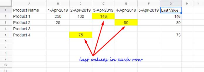
Let’s start with an example where the data is distributed across the range A1:F, and our goal is to find the last number in each row from B2:F2, B3:F3, B4:F4, and so on.

In the following screenshot, you can see that in column G, I have extracted the last values from each row.

The values in consideration are numeric.

Now, let’s delve into the non-array formula first.

Non-Array Formula:

In cell G2, input the following XLOOKUP formula, and then drag the fill handle (a small square in the bottom-right corner of the cell) downward:

=ArrayFormula(XLOOKUP(TRUE, ISNUMBER(B2:F2), B2:F2,,0,-1))

This formula returns the last number in each row. In case a row is blank, it will yield a null result.

How does this formula function?

Syntax of the XLOOKUP function:

XLOOKUP(search_key, lookup_range, result_range, [missing_value], [match_mode], [search_mode])

In our formula:

• search_key: TRUE
• lookup_range: ISNUMBER(B2:F2) – We utilize the ISNUMBER function, which returns TRUE if a cell contains a number; otherwise, it returns FALSE. Therefore, our search_key is TRUE. The ISNUMBER function checks whether a value is a number. Since we apply this to a row, we use the ARRAYFORMULA function in conjunction with XLOOKUP.
• result_range: B2:F2
• missing_value: Left blank to return null if no matches are found.
• match_mode: 0 for an exact match.
• search_mode: -1 to match from the last value to the first value.

The formula extracts the last non-blank value in a row with this setup.

Array Formula:

We aim to extract the last number in each row using the BYROW function with XLOOKUP in Google Sheets.

This function allows the G2 formula to expand downward automatically, eliminating the need to manually drag the fill handle. Let’s delve into the formula and then proceed with an explanation.

Scalable Array Formula:

Enter the formula in G2; it will expand to G3:G if G3:G is blank; otherwise, it returns a #REF error.

=ArrayFormula(BYROW(B2:F, LAMBDA(r, XLOOKUP(TRUE, ISNUMBER(r), r,,0,-1))))

Syntax of the BYROW Function:

BYROW(array_or_range, lambda)

The ‘lambda’ function creates a custom operation.

Syntax of the LAMBDA Function:

LAMBDA([name, …], formula_expression)

The final syntax is:

BYROW(array_or_range, LAMBDA([name, …], formula_expression))

Where:

• array_or_range: B2:F – the range to extract the last number from each row.
• name: r – represents the current row element.
• formula_expression: XLOOKUP(TRUE, ISNUMBER(r<>), r,,0,-1)) where ‘r’ signifies the current row.

In summary, this formula utilizes the BYROW function along with a lambda function to iterate through each row (designated by ‘r’) in the specified range (B2:F), employing XLOOKUP to find the last non-blank number in each row.

Formulas for Retrieving the Last String in Each Row in Google Sheets

In all the examples above, the formulas are designed to retrieve the last number in each row, focusing on columns containing numeric values.

If you wish to adapt these formulas to return the last string in each row, a single modification is needed.

Replace the ISNUMBER function with ISTEXT, and here are the adjusted array and non-array formulas for extracting the last string in each row:

Non-Array Formula:

=ArrayFormula(XLOOKUP(TRUE, ISTEXT(B2:F2), B2:F2,,0,-1))

Insert it in cell G2 and drag it down.

Scalable Array Formula:

=ArrayFormula(BYROW(B2:F, LAMBDA(r, XLOOKUP(TRUE, ISTEXT(r), r,,0,-1))))

Insert it in cell G2, and let the formula expand down dynamically.

Note: These two formulas won’t differentiate between numbers, dates, timestamps, or time.

Additional Tip: Extract the Last Value in Each Row Regardless of Data Type

In the above formulas, we have utilized ISNUMBER(B2:F2) or ISTEXT(B2:F2) in non-array formulas and ISNUMBER(r) or ISTEXT(r) in array formulas to extract the last number or text in each row.

If you prefer to extract the last value irrespective of data type, use B2:F2<>"" or r<>"" instead.

Sample Sheet

Resources

Understanding how to find the last value in each row in Google Sheets is crucial for effective data analysis.

Utilizing a combination of non-array and array formulas, such as XLOOKUP with ISTEXT or ISNUMBER, empowers users to tailor their approach based on different data types.

These formulas offer flexibility, allowing for dynamic extraction that can easily adapt to diverse datasets.

Whether you’re seeking the last number, text, or any value, these versatile tools enhance your ability to analyze data within Google Sheets.

Here are some additional resources that you might find interesting.

1. Google Sheets: How to Return First Non-blank Value in A Row or Column.
2. XMATCH First or Last Non-Blank Cell in Google Sheets
3. Find the Cell Address of a Last Used Cell in Google Sheets.
4. How to Find the Last Row in Each Group in Google Sheets.
5. Find the Last Entry of Each Item from the Date in Google Sheets.
6. Find the Average of the Last N Values in Google Sheets.
7. How to Find the Last Matching Value in Google Sheets.
8. How to Lookup First and Last Values in a Row in Google Sheets
9. Extract the Last Value from Each Column in Google Sheets
10. Lookup Last Partial Occurrence in a List in Google Sheets.