You can follow these tips regardless of your data orientation—whether it’s in rows or columns. I’ve got the solution for you! You can find the average of the last n values in Google Sheets using my flexible formula below.
Why flexible? Because it allows you to include or exclude 0s in the average calculation and automatically skips empty cells while selecting n values.
I’ll provide different formulas for horizontal and vertical datasets. You may need to tweak the formulas slightly based on whether you want to include or exclude 0s and depending on your data’s orientation.
Find the Average of the Last N Values in a Column
In this example, I want to calculate the average of the last 4 values in the range B1:B.
Excluding 0s
Here’s the formula for excluding 0s:
=LET(range, FILTER(B1:B, B1:B>0), n_rows, CHOOSEROWS(range, SEQUENCE(4, 1, -1, -1)), AVERAGE(n_rows))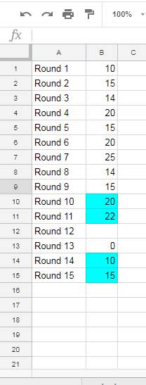
Including 0s
To include 0s, replace B1:B>0 with LEN(B1:B) in the formula:
=LET(range, FILTER(B1:B, LEN(B1:B)), n_rows, CHOOSEROWS(range, SEQUENCE(4, 1, -1, -1)), AVERAGE(n_rows))Adjusting the Formula for Your Needs
- Replace
B1:B: Use the range containing your values. - Adjust
4inSEQUENCE(4,...): This controls n. For example, to calculate the average of the last 10 values, replace4with10.
Formula Explanation
Excluding 0s:
FILTER(B1:B, B1:B>0): Filters the range to exclude empty cells and0s. In the formula, this is named asrangeusing LET.CHOOSEROWS(range, SEQUENCE(4, 1, -1, -1)): Extracts the last 4 rows from the filtered range. This result is stored inn_rows.AVERAGE(n_rows): Calculates the average of the last 4 rows.
Including 0s:
FILTER(B1:B, LEN(B1:B)): Filters the range to include all non-empty cells, including0s.- The remaining steps are the same as above.
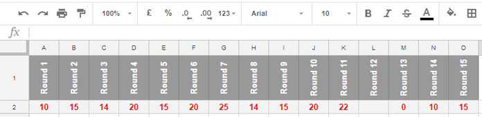
Find the Average of the Last N Values in a Row
Let’s adapt the formula for a horizontal dataset, such as values in A2:O2 or the entire row A2:2.
Key Changes
- Replace the column range (
B1:B) with the row range (A2:2). - Replace CHOOSEROWS with CHOOSECOLS.
Excluding 0s:
=LET(range, FILTER(A2:2, A2:2>0), n_rows, CHOOSECOLS(range, SEQUENCE(4, 1, -1, -1)), AVERAGE(n_rows))Including 0s:
=LET(range, FILTER(A2:2, LEN(A2:2)), n_rows, CHOOSECOLS(range, SEQUENCE(4, 1, -1, -1)), AVERAGE(n_rows))Conclusion
In this tutorial, you learned how to calculate the average of the last n values in both rows and columns in Google Sheets.
Including or excluding 0s can significantly impact your average calculations. Cells containing 0s are counted in the divisor for average calculations, which may skew your results. My formulas provide the flexibility to handle both scenarios effectively.


Thank you for this article. This is just what I’ve been looking for.
I want to average the last 5 entries of my row. You can see a sample here: link removed by admin
But it tells me the average is 3.84 when it should be 3.9.
Can you help?
Hi, Reagan Amaranson,
It’s because cell AE1 is empty. The header row must contain field labels in all the columns.
Thank you so much! That solved it!
Works like a charm!
Thank you for sharing 🙂
What would I need to change to make the calculation of the mean of N be from the front side of a row of scores…I will add a new score column each week in the same column (E) and push the older scores to the right….this is the formula I have working for now but it computes the mean of the last 3 scores…I want this so that the newest scores are in the front of the spreadsheet.
=ArrayFormula(iferror(average(query(transpose(if(len(E2:2),{COLUMN(E2:2);E3:3},)),"Select Col2 where Col2>0 order by Col1 Desc limit 3"))))Hi, Marc Z,
Use the Array_Constrain to constrain the rows and use average on them.
Syntax:
=average(ARRAY_CONSTRAIN(E2:E,n,1))Thank you. This does average the first 3 numbers, however…the exclusion of “0” or blanks is removed…how do I get that back in there?
tyia
Hi, Marc Z.
By including Filter() as below.
=average(ARRAY_CONSTRAIN(filter(E2:E,E2:E>0),n,1))Hey, thanks for the above btw, amazing stuff.
I am trying to get this formula working and have had some success.
I have two problems though, how do I get it to only ignore blank cells but include 0s?
Also, I would like to return the average in the same row as the data. However, I get “Circular dependency detected. To resolve with iterative calculation, see File > Spreadsheet settings.”
Should I adjust this setting or should I be updating one of the ranges so that it stops before the cell containing the formula?
Any help would be really appreciated.
Hi, Cameron,
If I know the data range and the cell in which you wish to key the formula in, I would be able to help you (or share the URL of a mockup sheet).
Hi,
I am trying to get a rolling 42-day average and include days for which there is no entry.
The entries so far I only have entries for 10 day so when I apply
=ArrayFormula(average(indirect("B"&MATCH(2,1/(B1:B<>""),1)+1-42&":B"&MATCH(2,1/(B1:B<>""),1))))there is a problem, cannot have a B0 cell.Is it possible to increase the range on the average to the up last entry then roll the average after 42 days?
Hi, Nick,
Your numbers to find the rolling average are in B1:B where B1 contains a label.
So I assume the numbers are in B2:B and here is my formula.
=average(query(ArrayFormula({indirect("B2:"&"B"&MATCH(2,1/(B1:B<>""),1)),row(indirect("B2:"&"B"&MATCH(2,1/(B1:B<>""),1)))}),
"Select Col1 order by Col2 desc limit 42"))
This formula will return the average of the numbers in B2:B, if the count of numbers is less than or equal to 42. Else it would return the rolling average of the last 42 numbers.
The above formula would exclude blanks. To include blanks, additionally use the function N with the above formula. It would be;
=ArrayFormula(average(N(query({indirect("B2:"&"B"&MATCH(2,1/(B1:B<>""),1)),row(indirect("B2:"&"B"&MATCH(2,1/(B1:B<>""),1)))},
"Select Col1 order by Col2 desc limit 42"))))
I hope these formulas help?
Hello, I have a running closing price sheet that pulls price from 1 to 30 days, but it also pulls week-ends!! which messes up the SMA calculation as they repeat the Friday closing price on Saturday and Sunday.
How do I eliminate weekends which mess up the average as they are repeated values? I am trying to compare the SMA 10 vs SMA 20.
Hi, Fernando Davidez,
You want to do two things – excluding weekends (Saturday and Sunday) then extract last ‘N’ values.
So obviously you have a date column that makes our task easy as we can sort this column in Z-A order for the last ‘N’ values.
Let’s assume the range is A2:B and A2:A contains dates. In my example, the ‘N’ is 10.
You can either use the Filter or the relatively simple Query to extract the values.
Filter
=array_constrain(filter(sort(B2:B,A2:A,0),(weekday(sort(A2:A,1,0))<>1)*(weekday(sort(A2:A,1,0))<>7)),10,1)Query
=query({A2:B},"Select Col2 where dayofweek(Col1)<>7 and dayofweek(Col1)<>1 order by Col1 desc limit 10")Wrap the above formulas with the average()
Hi. I’m trying to avoid adding formulas using Google Apps Script. However, that’s a possibility if my idea doesn’t work.
I’ve got a sheet where a new blank row is added at the bottom each week. I need to average the last n values in a specific column (column E) and return the result in column L.
For example, here is the sequence of events: (Column headers are in Row 1)
Row 2 is added, and a value is put in cell E2, all by script
Row 3 is added, and a value is put in cell E3, all by script
An average of E2:E3 is calculated and put in cell L3
Row 4 is added, and a value is put in cell E4, all by script
An average of E3:E4 is calculated and put in cell L4
Row 5 is added, and a value is put in cell E5, all by script
An average of E4:E5 is calculated and put in cell L5
This sequence of events continues each week, with the sheet getting a new tab each year. Currently, I am processing other data in other columns, and each column’s “arrayformula” formula will evaluate the data in each new row created each week.
Should I add formulas by the script instead? If I use an arrayformula, what is the formula that I should use?
Hi, Kent Lassolet,
I have a formula in mind (involves Hlookup and MMULT). I’ll test it and let you know. But I have no problem sharing the logic right now.
I’ll split/copy every two numbers to columns based on the tips provided on this post – Move Single Column to Multiple Columns Using Hlookup in Google Sheets.
Then transpose the results and MMULT/2. That would be the required average results in a column.
I may require to find a way to distribute it to the correct row by inserting one blank cell below each value in the above result. I need to work on this last part.
I’ll update you soon.
Here is the said tutorial – Array Formula to Return Average of Every N Cells in Google Sheets.
I’m using Sheets to track Blood Sugar for diabetes, BP, and weight.
Cannot figure out the edits to get an AVG Sugar reading for the last 7, 30, 60, 90 entires.
Sugars read Start ColB, Row3.
Thanks
Hi, Stephen Harris,
To calculate the average of the last 7 entries, use the below Average + Query combo.
=average(IFERROR(query(sort(B3:B,row(A3:A),0),"Select * where Col1>0 limit 7")))Change
limit 7tolimit 30to get the average of the last 30 entries. I hope you can follow this to get the average of the last 60 as well as 90 entries.PERFECT!!!
Thanks for assist!!
Hi there,
I have a dataset that runs from B378 to B458 and I want to be able to average the last n lot of values. When I used the formula you offered to “James” above but keep getting “#DIV/0” as my answer. All I did to the above formula was change the “B1:B” to “B378:B458”. Could you please show me the correct formula I should be using.
Thanks
Hi, Xavier,
Also change
row(A1:A)torow(A378:A458).If you still have issues, please feel free to make a sample file (sheet) and share it with your comment/reply.
Thanks for the reply. I have ten columns of separate data starting at B378:B458 and going across to K378:K458. I have the formula under each column changed accordingly. It works for 6 out of 10 columns but the other 4 have a
#DIV!0output. Is there any reason this might happen.Thanks for any help you could offer me.
Hi, Xavier,
Do those columns format as ‘plain text’ (Format menu > Number)?
If not, it’s high time to consider sharing a copy (sample data only) of your sheet contains the problem.
What if I want to include blanks and 0s?
Hi, Mike,
To include blanks and 0s in last n average, use the below formula.
=ArrayFormula(average(indirect("B"&MATCH(2,1/(B1:B<>""),1)+1-4&":B"&MATCH(2,1/(B1:B<>""),1))))This is for column B. For column C, change all the capital letters B in the formula to C.
Change the number 4 to 10 for the mean of the last 10 numbers.
Hi. I have an issue but not sure if this is the correct place to post it. I have two columns in Google Sheets. One for Names and one for Results. Example:
Name | Results
John | 1
Bill | 0
Susan | 1
John | 0
There are hundreds of rows like this. I’m looking for a way to find the average of the last number of results for a name.
For example, I want to know the average of the last 10 results for John. Do you know a formula for how to do this? Thanks for your help.
Hi, John,
Yes! I do have a formula. Please check this new tutorial – Formula to Conditionally Filter Last N Rows in Google Sheets.
Can you help me? I only need one column to be added. How do I use this formula with only one column (not 2)?
Something like this?
=ArrayFormula(iferror(average(query(B1:B,"Select Col2 where Col2>0 order by Col1 Desc limit 4"))))To calculate the MEAN of last ‘n’ values (here n=4) leaving 0s and blanks, you can use this new formula.
=average(IFERROR(query(sort(B1:B,row(A1:A),0),"Select * where Col1>0 limit 4")))This formula only requires the column that contains the values to average.
I need help! I have tried to use this and I can’t make it work.
I need to calculate the last 10 days average in column D and the date is in column A. I also need to exclude the blanks but include a zero.
Hi, Susan,
Formula:
=average(query({A2:A,D2:D},"Select Col2 where Col2>=0 order by Col1 Desc limit 10"))Excluded the title row (here row#1) in the selection.
If this doesn’t work, please share your Dataset (Sample only).
Best,