AVERAGEIFS Array Formula by Date Range in Google Sheets

If you’ve ever tried to calculate average values based on a list of dates in Google Sheets, you probably ran into a wall with AVERAGEIFS. It’s great for conditional averages—but only one at a time. And if you want to fill down for multiple dates, you end up copy-pasting the same formula again and again.

Not ideal, especially when your data keeps growing.

In this tutorial, I’ll show you how to write an AVERAGEIFS array formula by date range in Google Sheets that expands automatically—no dragging, no duplication. It’s clean, efficient, and perfect for calculating something like average daily rate (ADR) for hotel bookings or any date-based metric.

Let’s start with a simple dataset and work our way through the formula.

Table of Contents

Sample Data Setup

I’m using a basic hotel booking dataset. Columns A and B have the arrival and departure dates. Column C calculates how many nights were booked. Then we have the number of rooms in D, total revenue in E, and the average daily rate (ADR) in F.

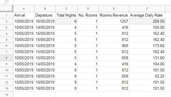
Hotel booking sample data with arrival and departure dates, rooms, revenue, and calculated ADR in Google Sheets

Total Nights Formula

In cell C2, we calculate the number of nights with:

=ArrayFormula(IF(A2:A, DAYS(B2:B, A2:A), ))

ADR Formula

Since the revenue spans multiple nights and rooms, the correct ADR formula in F2 is:

=ArrayFormula(IFERROR(E2:E / D2:D / C2:C))

That sets up our data. Now, let’s move to the actual formulas.

Step 1: Define Your Date Criteria

In column H, enter the list of dates you want to check against. These are the dates you’ll calculate average rates for.

Step 2: Try the Non-Array Version First

To understand what we’re calculating, start with a regular AVERAGEIFS formula in I2, then copy it down:

=IFERROR(AVERAGEIFS($F$2:$F$13, $A$2:$A$13, "<=" & H2, $B$2:$B$13, ">" & H2))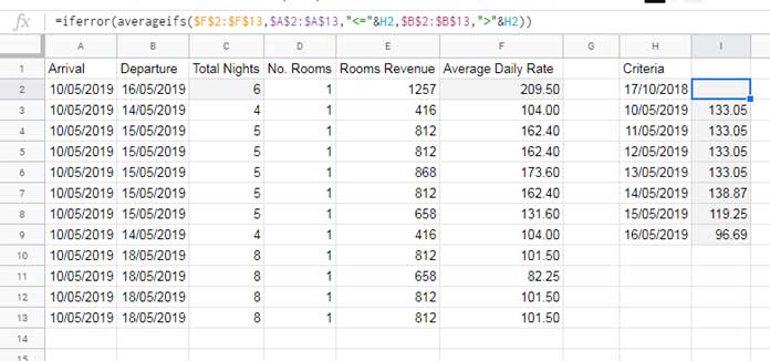

AVERAGEIFS formula by date range in Google Sheets shown using manual drag-down across multiple rows

This formula checks for all bookings that were active on the date in H2—that is, where the arrival date is on or before the date, and the departure date is after it. It then returns the average of the ADR values from column F for those matching bookings.

But again, you have to drag the formula down for each row in column H. Let’s fix that.

Step 3: AVERAGEIFS as an Array Formula

Replace all the formulas in column I with this one formula in I2:

=MAP(H2:H, LAMBDA(r, IFERROR(AVERAGEIFS(F2:F, A2:A, "<=" & r, B2:B, ">" & r))))

How the Formula Works

MAP loops through each date in column H
LAMBDA plugs each date (r) into the formula
AVERAGEIFS does the filtering and averaging
IFERROR handles blank or unmatched dates

It’s simple, fast, and works with expanding criteria ranges.

Sample Sheet

Optional: The Old MMULT Trick

Before MAP came along, you could get this done using MMULT, TRANSPOSE, and some matrix math. It works, but it’s slower and harder to follow.

Here’s what that formula looks like:

=ArrayFormula(IFERROR(
  IF(H2:H="",,
    MMULT(((TRANSPOSE(A2:A) <= H2:H) * (TRANSPOSE(B2:B) > H2:H)), N(F2:F)) /
    MMULT(((TRANSPOSE(A2:A) <= H2:H) * (TRANSPOSE(B2:B) > H2:H)), ROW(A2:A)^0)
  ), 0))

Unless you really enjoy array gymnastics, I’d recommend sticking with MAP. It’s cleaner and more maintainable.

Wrapping Up

That’s how you build an AVERAGEIFS array formula by date range in Google Sheets—no dragging, no repetition, and fully dynamic. It’s a great way to calculate daily averages from time-based data like bookings, attendance, or usage logs.