Want to calculate the average of every N cells in a column in Google Sheets using a single array formula?
This tutorial shows you how to do just that — without using Apps Script or helper columns.
This technique is helpful in many real-world scenarios.
For example, if you collect data points like daily sales or temperature readings, you might want to calculate weekly or hourly averages to better understand trends. In such cases, you can enter the values in a column and use an array formula to average every N cells in that column automatically.
Averaging every N cells helps smooth noisy data or plot group-level summaries without needing pivot tables or helper columns.
Modern Array Formula to Average Every N Cells in Google Sheets
This cleaner method uses LET, WRAPROWS, and BYROW to group and average every N values:
Assume you have the sample data in the range E2:E, and you define n in cell H2.
Then use the following formula in cell F2 to calculate the average of every N cells:
=LET(
   range, E2:E,
   n, H2,
   avg, BYROW(WRAPROWS(range, n), LAMBDA(r, AVERAGE(r))),
   pad, WRAPROWS(,n-1),
   fnl, IF(n=1, range, IFERROR(TOCOL(HSTACK(pad, avg)))),
   fnl
)
The formula calculates the average of every N cells and pads (N – 1) empty cells between each result, so the output stays aligned with the original data length.
How It Works
1. BYROW(WRAPROWS(range, n), LAMBDA(r, AVERAGE(r)))
The WRAPROWS function wraps the single-column range into rows of n columns. So if n = 3, each row will contain 3 cells.
The result:
| 10 | 20 | 25 |
| 60 | 5 | 6 |
| 7 | 8 | 10 |
| 30 | 65 | 50 |
| 45 | 0 | 0 |
| 0 | 0 | 8 |
Then BYROW applies AVERAGE to each row, returning:
18.33
23.67
8.33
48.33
15.00
2.67
That’s the average of every N cells.
Tip: If you only want this output, replace fnl (the very last one) with avg in the formula.
2. pad
WRAPROWS(,n-1) returns the padding cells needed to align with the input data shape.
3. fnl
This part returns the final result:
IF(n=1, range, IFERROR(TOCOL(HSTACK(pad, avg))))- If
n = 1, it just returns the original range. - Otherwise, it stacks padding and averages, then flattens into a single column.
That’s your final array formula to average every N cells in Google Sheets.
Legacy Array Formula to Average Every N Cells (Pre-LET and BYROW)
Before LET, BYROW, and WRAPROWS, we used this complex formula:
=ArrayFormula(IFNA(VLOOKUP(IF(MOD(SEQUENCE(MROUND(COUNT(E2:E), H2), 1), H2)=0, COUNTIFS(MOD(SEQUENCE(MROUND(COUNT(E2:E), H2), 1), H2), MOD(SEQUENCE(MROUND(COUNT(E2:E), H2), 1), H2), SEQUENCE(MROUND(COUNT(E2:E), H2), 1), "<="&SEQUENCE(MROUND(COUNT(E2:E), H2), 1)),), {SEQUENCE(MROUND(COUNT(E2:E), H2)/H2, 1), ARRAY_CONSTRAIN(MMULT(N(IFERROR(HLOOKUP("test", E1:E, SEQUENCE(ROUNDUP(COUNTA(E1:E)/H2), H2, 2), 0))), SEQUENCE(H2, 1)^0)/H2, COUNT(SEQUENCE(MROUND(COUNT(E2:E), H2)/H2, 1)), 1)}, 2, 0)))Here are the steps that formula breaks into:
1. Re-Arrange a Single Column into Multiple N Columns
=ArrayFormula(IFERROR(HLOOKUP("test", E1:E, SEQUENCE(ROUNDUP(COUNTA(E1:E)/H2), H2, 2), 0)))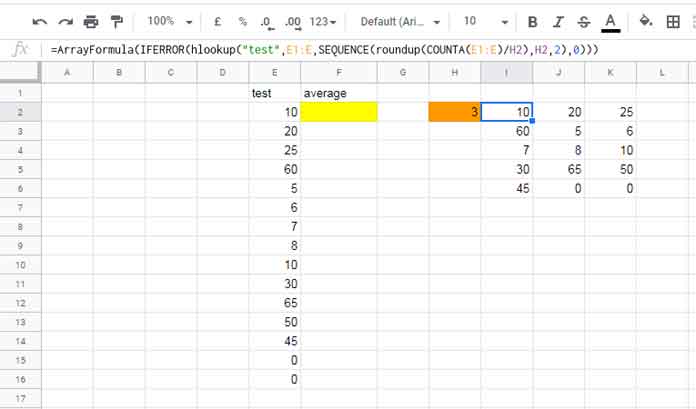
2. Row-Wise Average Using MMULT
Remove the Step 1 formula and enter the following in cell J2:
=ArrayFormula(MMULT(N(IFERROR(HLOOKUP("test", E1:E, SEQUENCE(ROUNDUP(COUNTA(E1:E)/H2), H2, 2), 0))), SEQUENCE(H2, 1)^0)/H2)Now trim the result based on the source data using ARRAY_CONSTRAIN:
=ArrayFormula(ARRAY_CONSTRAIN(MMULT(N(IFERROR(HLOOKUP("test", E1:E, SEQUENCE(ROUNDUP(COUNTA(E1:E)/H2), H2, 2), 0))), SEQUENCE(H2, 1)^0)/H2, COUNT(SEQUENCE(MROUND(COUNT(E2:E), H2)/H2, 1)), 1))3. Generate Sequence for Row Indexing
=SEQUENCE(MROUND(COUNT(E2:E), H2)/H2, 1)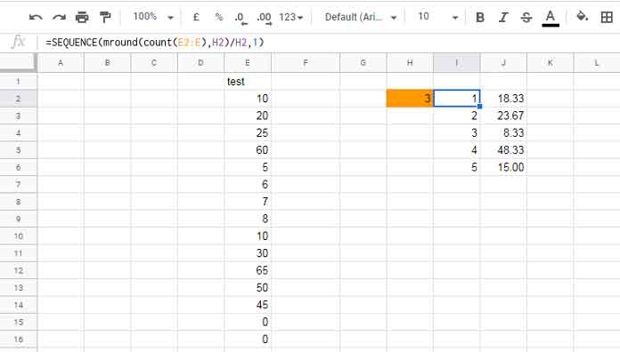
4. Mark Every Nth Cell
=ArrayFormula(MOD(SEQUENCE(MROUND(COUNT(E2:E), H2), 1), H2))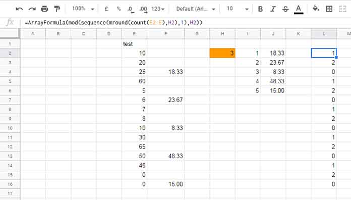
5. Running Count of Markers
=ArrayFormula(IF(INDIRECT("L2:L"&MROUND(COUNT(E2:E), H2)+1)=0, COUNTIFS(L2:L, L2:L, ROW(L2:L),"<="&ROW(L2:L)),))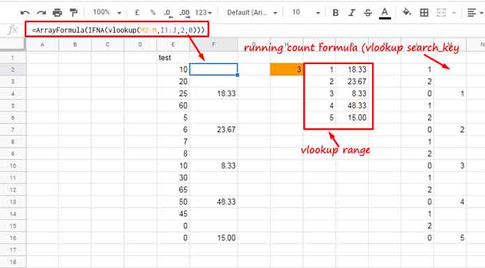
6. VLOOKUP to Distribute Averages
=ArrayFormula(IFNA(VLOOKUP(M2:M, I1:J, 2, 0)))We combine all these into the legacy array formula.
Note: You may want to keep a few extra rows (n extra) at the end of the values in column E. Also ensure the total number of values is a multiple of n.


