Are you using the GOOGLEFINANCE function to fetch historical data from Google Finance? Then you might want to learn how to calculate the Simple Moving Average (SMA) in Google Sheets.
However, the formula provided in this tutorial is not limited to securities data retrieved from Google Finance. I used the GOOGLEFINANCE function to import some historical data for demonstration purposes.
The formula simply requires a set of data points (numbers) in a column to work.
SMA: Understanding the Term
The Simple Moving Average (SMA) is the average of a fixed number of recent data points, updated every time new data becomes available. It’s one of the most basic and widely used tools in data analysis and financial markets to identify trends or underlying patterns.
To calculate the SMA, you add up the most recent n data points (e.g., closing prices for stocks) and divide the total by n.
We’ll use the GOOGLEFINANCE function to fetch closing prices for a specific ticker symbol over a given period and calculate the SMA. (You’re not limited to this; you can use your own data.)
First, let’s explore SMA with a simple example.
Basic Example of Calculating SMA in Google Sheets
Here’s an example of calculating the SMA for the last three data points in a range in Google Sheets.
In cell C3, I calculated the average of the last three data points in column A using the following formula:
=AVERAGE(A6:A8)When a new value becomes available in cell A9, we drop the oldest data point (A6) and include the new one (A9). This is reflected in the updated formula:
=AVERAGE(A7:A9)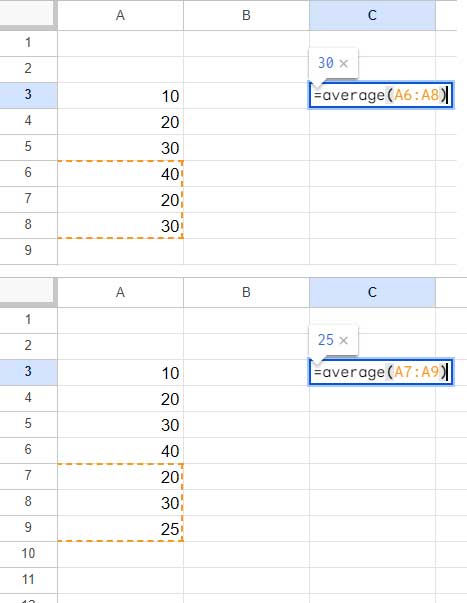
This demonstrates how SMA updates dynamically as new data is added. But how can we automate this process to avoid manually adjusting the range each time?
How to Calculate the Simple Moving Average Dynamically in Google Sheets
To calculate the SMA dynamically, you need a formula that can automatically extract the last n values in a column. Let’s assume your values are in column A. Here’s a dynamic formula to calculate the SMA:
=LET(range, A1:A, n, 3, ArrayFormula(IFERROR(AVERAGE(QUERY(IF(LEN(range), HSTACK(ROW(range), range), ), "SELECT Col2 WHERE Col2 > 0 ORDER BY Col1 DESC LIMIT " & n)))))In this formula:
nrepresents the number of recent values to include (in this case, 3).- The formula extracts the last n non-blank values in the column and calculates their average.
Formula Explanation
LET:
Assigns names (rangeandn) to improve readability and efficiency.range: Refers to the data inA1:A.n: Represents the number of values to consider, here set to 3.
IF(LEN(range), HSTACK(ROW(range), range), ):
Creates a two-column array:- The first column contains the row numbers of non-blank cells.
- The second column contains the corresponding values from the
range.
QUERY:
Selects the most recent n non-blank rows:- Filters out blank cells.
- Sorts the data by row numbers in descending order.
- Limits the output to the first n values.
AVERAGE:
Computes the average of the selected values returned by theQUERY.
Calculating SMA with GOOGLEFINANCE Data in Google Sheets
Let’s dynamically calculate the Simple Moving Average using historical stock data fetched with the GOOGLEFINANCE function in Google Sheets. SMA is a key component of trading strategies, helping to assess whether an asset’s price will continue its trend or reverse. It smooths out daily price fluctuations for clearer trend analysis.
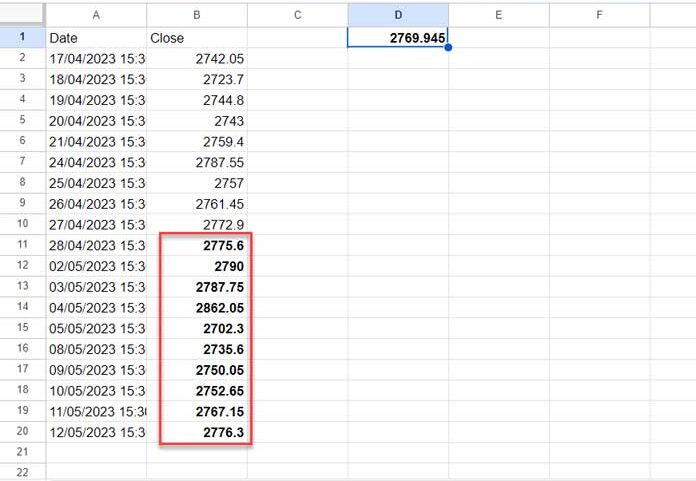
For example, we’ll calculate the SMA of the last 10 closing prices for HDFCBANK. To ensure sufficient data, import at least 30 days of historical data, as stock markets may have non-trading days.
Syntax of GOOGLEFINANCE:
GOOGLEFINANCE(ticker, [attribute], [start_date], [end_date|num_days], [interval])Formula to Fetch Data:
=GOOGLEFINANCE("HDFCBANK", "close", TODAY()-30, TODAY(), "daily")When entered in cell A1 of an empty sheet, this formula returns two columns: timestamps (column A) and closing prices (column B).
Note: This formula may or may not return historical data during your testing, depending on the availability of the ticker symbol. Ticker symbols can change or be removed over time. For testing, you can use any valid ticker symbol available on the Google Finance website.
Formula to Calculate SMA:
Modify the previous SMA formula to fit this data:
- Replace
n(3) with10. - Replace
A1:AwithB1:B.
=LET(range, B1:B, n, 10, ArrayFormula(IFERROR(AVERAGE(QUERY(IF(LEN(range), HSTACK(ROW(range), range), ), "SELECT Col2 WHERE Col2 > 0 ORDER BY Col1 DESC LIMIT " & n)))))Now, this formula dynamically calculates the SMA for the last 10 closing prices in column B.
Note: You can specify B1:B (including the header) or B2:B (excluding the header). The QUERY function is capable of identifying and handling the header row automatically, so the result will be the same in either case.
Conclusion
The above formula is one way to calculate the SMA in Google Sheets. If your data is arranged in rows instead of columns, you can transpose it or use a modified formula. Since the core logic involves identifying the last n values and wrapping them with the AVERAGE function, you might also explore alternatives like How to Find the Average of the Last N Values in Google Sheets.
Resources
- Array Formula to Return Average of Every N Cells in Google Sheets
- Calculating Running Average in Google Sheets
- Calculating Rolling N Period Average in Google Sheets
- Reset Rolling Averages Across Categories in Google Sheets
- Google Sheets: Rolling Average Excluding Blank Cells and Aligning
- Dynamic Moving Average in Excel
- Dynamic Weekly Averages in Excel Without Helper Columns


Hi,
How to do EMA instead of SMA and MACD Histogram? Essentially, I want to do the Elder impulse calculation.
Thanks
Any chance in providing an example google sheets with the above in it? I’m having a difficult time grasping the above.
Would there be a way to use your dynamic formula but rather than point to a specific stock within the formula, point to a cell instead.
Then that cell would contain a stocks ticker symbol? Then you could just copy that formula down the page for a list of hundreds of stocks, rather than replacing each stock within the formula?
Hi, Phillip Batch,
That you can do as below.
Enter the ticker symbols in A1:A. Then use this GoogleFinance formula in cell C1.
=GOOGLEFINANCE(A1,"close",today()-30,today())Now, modify the above formula in cell C1 to include the Query.
=Query(GOOGLEFINANCE(A1,"close",today()-30,today()),"Select Col2 where Col2 is not null order by Col1 desc limit 10 label Col2''")This Query will return historical data for the last 10 days. Here instead of using the ROW function, I have sorted the historical data in descending order (the timestamp column) and limit the number of rows to 10.
Here is SMA
=iferror(average(Query(GOOGLEFINANCE(A1,"close",today()-30,today()),"Select Col2 where Col2 is not null order by Col1 desc limit 10 label Col2''")))You can copy this formula down to change the ticker.
your dynamic array formula is clever:) I was stuck with the disability of “array forumlating” the query function, but your is a much better generalisation given the query constraints!