This post guides you through calculating a rolling average while excluding blank cells and maintaining proper alignment in Google Sheets.

We can utilize an array formula based on the AVERAGE function to compute the rolling average of ‘n’ data points within a specified time frame in Google Sheets. Relevant formulas have been shared earlier, and links to those tutorials can be found in this post (assuming there are no blank cells).

The current focus is on calculating a rolling average while excluding blank cells and preserving alignment in Google Sheets.

This is crucial because the AVERAGE function disregards blank cells, leading to an inconsistency in the number of values within the specified time frame.

Let me illustrate this with a drag-down formula, although we’ll use an array formula in this tutorial for the final result.

Handling Blank Cells in Rolling Average Calculations: Clarifying the Issue

Consider a scenario involving a 3-day rolling average calculation applied to a dataset of stock prices.

Column A contains dates, and column B contains corresponding stock prices. Column C illustrates the rolling average calculation while emphasizing the blank cell issue.

While the days in column A follow sequential order, historical stock prices are available only for weekdays, resulting in blank cells in column B.

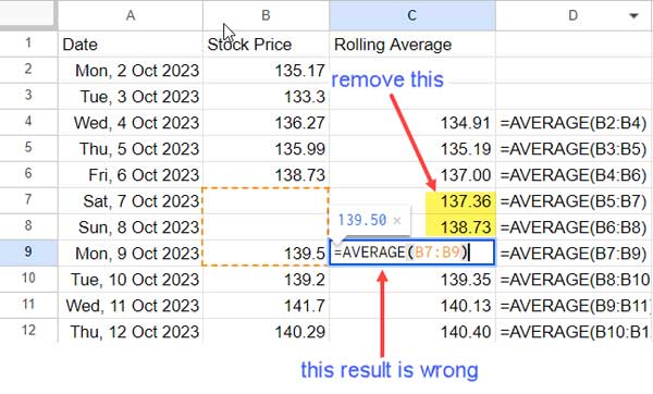
Despite the AVERAGE formula in cell C9 having a range of 3, it omits two blank cells, leading to an inaccurate 3-day rolling average. Additionally, we aim to exclude the result corresponding to blank cells.

I’ve inserted the following AVERAGE formula in cell C4, which has been copied down:

=AVERAGE(B2:B4)

Alternatively, you can utilize the following array formula in cell C2:

=MAKEARRAY(ROWS(B2:B), 1, lambda(r, c, IFERROR(AVERAGE(CHOOSEROWS(B2:B, SEQUENCE(3, 1, r-3+1))))))

You can find an explanation of this array formula in my previous tutorial titled “Calculating Rolling N Period Average in Google Sheets”

Both of these formulas won’t return the correct result due to the empty cells in column B. They are designed for use with a non-blank range.

Rolling Average Array Formula that Excludes Blank Cells and Aligns Results

Based on the above example, you can apply the following array formula in cell C2:

=MAP(B2:B, LAMBDA(cats, IF(cats="", ,IF(COUNTA(FILTER(B2:cats, B2:cats<>""))<3,, AVERAGE(CHOOSEROWS(FILTER(B2:cats, B2:cats<>""), SEQUENCE(3, 1, -1, -1)))))))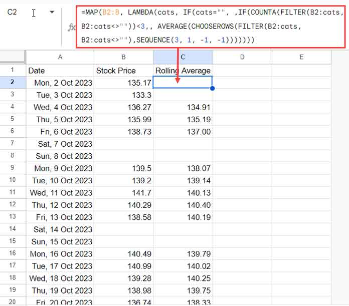

You can access the sample data and formula from my sample sheet below:

Sample Sheet

This is a rolling 3-day average excluding blank cells. To convert it to an n-day average:

For example, to change from 3-day to 5-day, replace the occurrences of 3 (which occur twice in the formula) with 5.

This formula excludes blank cells in the rolling average calculation and returns results skipping the blank cells.

This formula is entirely distinct from our earlier array formula (the MAKEARRAY one above), which was coded for datasets with non-blank cells.

Let’s explore how this function eliminates blank cells in the rolling average calculation, ensuring the accurate count of values in each rolling time frame, and observe how it also bypasses empty rows.

Formula Explanation

The MAP function in the provided formula expands a non-array formula result.

To achieve a rolling average that excludes blank cells and maintains alignment, we will first explore the non-array formula that should be entered into cell C2.

You can then copy-paste it down to apply the rolling average to the entire range. Once you grasp this non-array formula, understanding the MAP part will become much easier.

This is the non-array formula in cell C2:

=IF($B$2:B2="", , IF(COUNTA(FILTER($B$2:B2, $B$2:B2<>""))<3,, AVERAGE(CHOOSEROWS(FILTER($B$2:B2, $B$2:B2<>""),SEQUENCE(3, 1, -1, -1)))))

When you drag this formula down, the range $B$2:B2 adjusts as follows:

• In cell C3: $B$2:B3
• In cell C4: $B$2:B4
• In cell C5: $B$2:B5
• In cell C6: $B$2:B6
• In cell C7: $B$2:B7
• In cell C8: $B$2:B8
• In cell C9: $B$2:B9
• …

To understand the logic, let’s examine what happens in cell C9.

Rolling Average with Blank Cell Exclusion

Let’s break down each part and examine what happens in cell C9.

Section # 1:

=FILTER($B$2:B9, $B$2:B9<>"")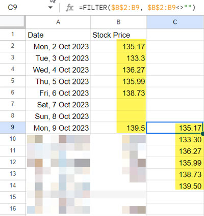

Syntax of the FILTER Function:

FILTER(range, condition1, [condition2, …])

Where:

• $B$2:B9: This is the range from which data is filtered.
• $B$2:B9<>"": This condition checks if each cell in the specified range is not equal to an empty string. It filters out the blank cells.

The FILTER formula returns non-blank cells in the range B2:B9, essentially providing the stock prices in B2:B9 while excluding blank cells.

Section #2:

Since we’re calculating a 3-day rolling average, we need the last three values in this range. To achieve this, we use the CHOOSEROWS function. Here is the relevant part of the formula:

=CHOOSEROWS(FILTER($B$2:B9, $B$2:B9<>""), SEQUENCE(3, 1, -1, -1))

Syntax of the CHOOSEROWS Function:

CHOOSEROWS(array, [row_num1, …])

Where:

FILTER($B$2:B9, $B$2:B9<>""): This is the array from which we extract the last three values, excluding blank cells.
row_num1, row_num2, row_num3: The SEQUENCE function generates the array {-1, -2, -3}, instructing CHOOSEROWS to return three values from the bottom since the numbers are negative. These values represent the row numbers to be selected from the array.

Section #3:

The AVERAGE function then calculates the average of these three values:

=AVERAGE(CHOOSEROWS(FILTER($B$2:B9, $B$2:B9<>""),SEQUENCE(3, 1, -1, -1)))

This represents the logic of the rolling average excluding blank cells.

The formula in cell C2 includes two logical tests that ensure the correct alignment of the results in rows. Let’s revisit the C2 formula to understand these tests.

Two Alignment Checks: Ensuring Proper Row Placement of Results

In the following C2 formula, we have previously discussed the green color highlighted part in three sections, explaining what happens in cell C9 when we drag it down to cell C9.

=IF($B$2:B2="", , IF(COUNTA(FILTER($B$2:B2, $B$2:B2<>""))<3,, AVERAGE(CHOOSEROWS(FILTER($B$2:B2, $B$2:B2<>""),SEQUENCE(3, 1, -1, -1)))))

The highlighted part ensures the exclusion of empty cells in the rolling average computation.

There are two logical tests in the formula to align the results:

1. IF(COUNTA(FILTER($B$2:B2, $B$2:B2<>""))<3,,: This test checks whether the filter has three values. If it evaluates to TRUE, the formula returns the average; otherwise, it leaves the cell blank. This logical test excludes results in the initial two rows for a 3-day rolling average, four rows in a 5-day rolling average, and so forth.
2. IF($B$2:B2="", ,: This logical test checks the stock prices in column B. If there is a value, it computes the rolling average; otherwise, it leaves the cell blank. This test helps the formula skip the empty rows.

The Role of the MAP Function in Calculating Rolling Average Excluding Blank Rows

Formula:

=MAP(B2:B, LAMBDA(cats, IF(cats="", , IF(COUNTA(FILTER(B2:cats, B2:cats<>""))<3,, AVERAGE(CHOOSEROWS(FILTER(B2:cats, B2:cats<>""), SEQUENCE(3, 1, -1, -1)))))))

Syntax of the MAP Function:

MAP(array1, [array2, …], lambda)

Where:

• B2:B is array1.
  • This is the range that the MAP function will iterate over.
• LAMBDA(cats, IF(cats="", ,IF(COUNTA(FILTER(B2:cats, B2:cats<>""))<3,, AVERAGE(CHOOSEROWS(FILTER(B2:cats, B2:cats<>""), SEQUENCE(3, 1, -1, -1)))))) is lambda.
  • cats is a parameter representing the current element in the iteration, which helps increment the range B2:B2 to B2:B3, B2:B4, and so forth.
  • It facilitates the expansion of the formula down the column.

Conclusion

Above, you can find both array and non-array formulas to calculate a rolling average, excluding blanks, in Google Sheets.

I recommend using the array formula as it dynamically adjusts when you delete or insert new stock prices in your data. The non-array formula serves the purpose of helping you understand the underlying logic.

That concludes our discussion for now. Thank you for your time and attention.

Related: Reset Rolling Averages Across Categories in Google Sheets