This post details the process of resetting a rolling average when a category changes, utilizing an array formula in Google Sheets.

A rolling average is a moving average used to calculate trends over short periods of time, such as one week, one month, every three months, and so forth. It involves generating a series of averages across various time frames within a dataset.

In one of my earlier tutorials titled “Calculating Rolling N Period Average in Google Sheets,” I shared an array formula.

Here, we will modify that formula to incorporate the “reset” feature, and it’s a relatively simple process.

To begin resetting the rolling average, we require a sample dataset in Google Sheets. Please refer to the following image for the sample data, and you can also utilize my sample sheet by clicking on the “Sample Sheet” button below.

Sample Sheet

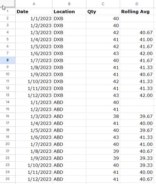
In the example above, in column D, you can observe that the rolling average is calculated for a 3-month time frame and resets when the category (Location) changes in column B.

Formula to Resetting Rolling Average in Google Sheets

Here is the formula that I’ve used in cell D2 in the example above:

=ArrayFormula(IF(
   COUNTIFS(B2:B, B2:B, ROW(B2:B), "<="&ROW(B2:B))<3, ,
   MAKEARRAY(ROWS(C2:C), 1, 
      lambda(r, c, 
      IFERROR(AVERAGE(CHOOSEROWS(C2:C, SEQUENCE(3, 1, r-3+1)))))
   )
))

How can I adjust the time frame for the rolling average in the formula above?

Replace the number 3, which occurs three times, with the desired number. To achieve a rolling average at every 4-month time frame that also resets at a category change, substitute all occurrences of the number 3 with 4. That’s it.

The detailed explanation of this formula follows after the formula logic below. I hope you will like that.

The Logic Behind Resetting Rolling Average in Google Sheets

To calculate the rolling 3-month average for each location, with the rolling average resetting when the area changes from DXB to ABD, follow these three main steps:

1. Obtain the running count of the category (location) column, determining when the rolling average resets.
2. Generate the rolling average using an array formula.
3. Apply an IF Logical statement to reset the rolling average based on the running count.

We will combine these three formulas into one, and it’s not a complex task.

The logic of the formula here is that we will eliminate the rolling average from rows where the running count returns the numbers 1 to 3, which will be equivalent to resetting.

If the time frame is 4 months, then you should eliminate the values in the rows where the running count returns the numbers 1 to 4.

Here are the step-by-step instructions for coding a formula that generates rolling averages with category resets in Google Sheets.

Running Count of Location

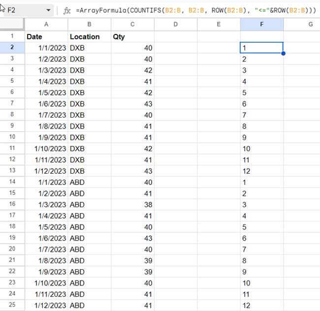
To generate the running count of locations, enter the following array formula in cell F2:

=ArrayFormula(COUNTIFS(B2:B, B2:B, ROW(B2:B), "<="&ROW(B2:B)))

This formula will return sequential numbers for each location, and the count will restart when the category (location) changes.

Anatomy of the Formula

Syntax of the COUNTIFS Function:

COUNTIFS(criteria_range1, criterion1, [criteria_range2, …], [criterion2, …])

The COUNTIFS Google Sheets function counts the number of cells in a range that meet multiple criteria.

• criteria_range1: B2:B
• criterion1: B2:B

It checks each cell in column B (from B2 to the end of the column) against itself.

If you simply use =ArrayFormula(COUNTIFS(B2:B, B2:B)), it will return the count of the categories DXB and ABD in each row, which will be 12.

To create a running count, a second set of conditions is needed:

• criteria_range2: ROW(B2:B)
• criterion2: "<="&ROW(B2:B)

This is where the interesting part comes in. The "<="&ROW(B2:B) part checks if the row number of each cell is less than or equal to its own row number.

This restriction ensures that the first set of criteria returns the total count up to the current row, not up to the last row and that is the running count.

Rolling Average of Quantity

Insert the following array formula into cell E2 to obtain the 3-month rolling average of quantities in column C:

=MAKEARRAY(ROWS(C2:C), 1, lambda(r, c, IFERROR(AVERAGE(CHOOSEROWS(C2:C, SEQUENCE(3, 1, r-3+1))))))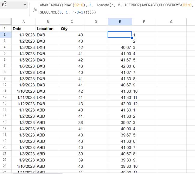

I have previously explained this unique formula in my tutorial. To find the link, please scroll up to the top where it is available in the third paragraph.

Here is a brief explanation before we reset these rolling averages across categories in Google Sheets:

The CHOOSEROWS function extracts 3 rows starting from cell C2, and the AVERAGE function calculates the average of these values.

=AVERAGE(CHOOSEROWS(C2:C, {1,2,3}))

We can replace {1,2,3} with SEQUENCE(3, 1, 1):

=AVERAGE(CHOOSEROWS(C2:C, SEQUENCE(3, 1, 1)))

The sequence starts at 1 and returns 3 numbers, i.e., {1, 2, 3}. By modifying the last number 1 (start argument) in SEQUENCE with 2, the sequence will start at 2 and return 3 numbers, i.e., {2, 3, 4}.

To automate this process, you can use a dynamic approach within the SEQUENCE function itself. Instead of hardcoding the start argument, we can use the MAKEARRAY function.

In other words, the following MAKEARRAY returns sequential numbers -1, 0, 1, 2, 3, 4 to n, up to the last cell in the sheet:

=MAKEARRAY(ROWS(C2:C), 1, lambda( r, c, r-3+1))

In this formula, r-3+1 is the formula_expression. We incorporate the aforementioned AVERAGE formula here and replace the start value in SEQUENCE with r-3+1.

The CHOOSEROWS will return errors in the first two cells because of the -1 and 0 returned by MAKEARRAY. The IFERROR function is used to handle and remove these errors.

The Role of IF Logical Statement in Resetting Rolling Average in Google Sheets

We will use the following generic formula to reset the rolling average in Google Sheets:

=ArrayFormula(IF(running_count_of_category<3, , rolling_average))

It essentially involves an IF logical test that incorporates a running count and a rolling average.

Here is the corresponding formula:

=ArrayFormula(IF(COUNTIFS(B2:B, B2:B, ROW(B2:B), "<="&ROW(B2:B))<3, ,MAKEARRAY(ROWS(C2:C), 1, lambda(r, c, IFERROR(AVERAGE(CHOOSEROWS(C2:C, SEQUENCE(3, 1, r-3+1))))))))

Where:

• running_count_of_category: COUNTIFS(B2:B, B2:B, ROW(B2:B), "<="&ROW(B2:B))
• rolling_average: MAKEARRAY(ROWS(C2:C), 1, lambda(r, c, IFERROR(AVERAGE(CHOOSEROWS(C2:C, SEQUENCE(3, 1, r-3+1))))))

Conclusion

We have explored the formula for resetting rolling averages across categories in Google Sheets.

You can make some improvements to the formula if you have categories and subcategories in two columns by combining them within the running count.

I am confident that this is a type of array formula that you may not be familiar with. Please leave your valuable feedback in the comments below.

Thanks for staying tuned. Enjoy!

Related: Google Sheets: Rolling Average Excluding Blank Cells and Aligning