Calculating rolling n-period averages is a common practice for analyzing data trends. How to write an array formula for this in Google Sheets?

Thanks to Google for introducing functions such as Lambda and Chooserows, which help to code, for example, a 7-day or 1-month rolling average array formula possible.

Rolling n period average and running average calculations are almost the same. They differ at one point and here it is.

The running average returns the average of something from the first date (assume you have a date column and value column in Google Sheets).

On the other hand, the rolling n-period average could look back at a specific time window, such as 7 days (one week) or 30 days (one month), and calculate the average continuously.

Another calculation is SMA which returns a single output. It’s the average of the recent n amount.

SMA can help traders in determining if an asset price will continue or if it will reverse a bull (upward) or bear (falling) trend.

Understanding Rolling N Period Average Calculation Using Drag-Down Formula in Google Sheets

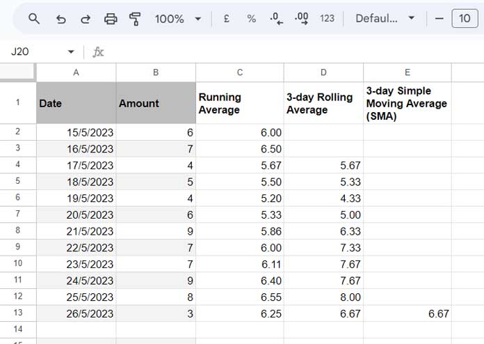
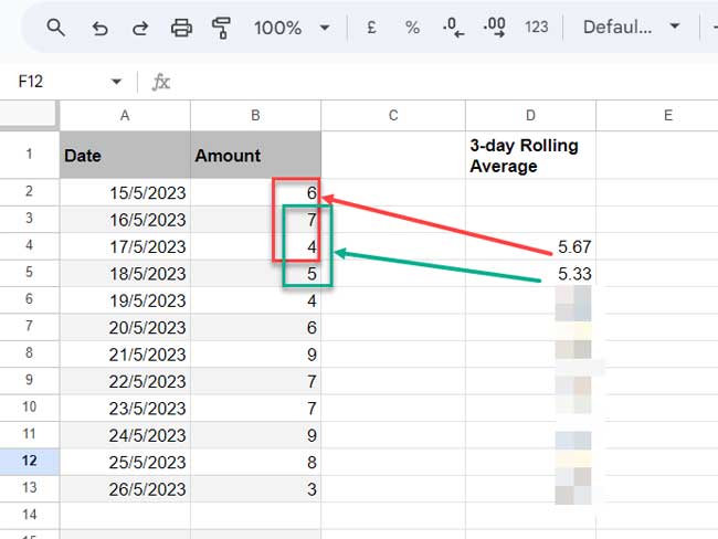
We will use the amounts in column B to calculate the rolling n-period average in Google Sheets (column D result).

We can use =average(B2:B4) in cell D3 and drag it down until D13 to get the rolling 3-day average in Google Sheets.

The syntax of the AVERAGE function is AVERAGE(value1, [value2, …]), where value1 can be a single value or a range.

In our case, it’s a range and B2:B4 in the cell D4 formula. As a side note, we don’t want to use the optional [value2, …] argument.

When we copy the D4 rolling average formula to the next cell down, i.e., D5, the range becomes B3:B5.

It helps us to get the rolling average of 3 sets of values. We aim to make it an array formula that sits in cell D2 and spills down.

Before going to that, here are the other two formulas (running average and SMA).

The following C2 formula returns the result in C2:C13 (please scroll up and see the first screenshot).

=byrow(B2:B,lambda(r,if(r="",,average(filter(B2:B,row(B2:B)<=row(r))))))

Please refer to Calculating Running Average in Google Sheets (Array Formulas).

The following E13 formula returns the result in E13 (please scroll up and see the first screenshot).

=ArrayFormula(iferror(average(query(if(len(A1:A),{ROW(A1:A),B1:B},),"Select Col2 where Col2>0 order by Col1 Desc limit 3"))))

Please refer to How to Calculate the Simple Moving Average in Google Sheets.

Calculating Rolling N Period Average Using Array Formula in Google Sheets

Array formulas usually require one or more blank rows or columns to spill their result.

Our rolling n-period array formula requires one blank column range D2:D13.

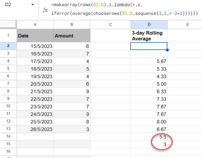
In cell D2, insert the following rolling 3-day array formula and see if it spills down the result.

=makearray(rows(B2:B13),1,lambda(r,c,iferror(average(chooserows(B2:B13,sequence(3,1,r-3+1))))))

How do we change rolling 3 to rolling n?

Please look at my above formula to see the number # 3 appears twice (the highlighted ones). Change them to 7 if you want a 7-day, to 30 for a 30-day rolling average in Google Sheets.

Can I Open the Range B2:B13?

You feel free to make the range B2:B13 open in the formula.

So B2:B13 will become B2:B, and you may get values in two more rows down. That is the result of the calculations =average(B12:B14) and =average(B13:B15).

Remember! We aim to calculate the rolling N period average using an array formula in Google Sheets.

In our above example, N = 3. So, the formula returns two additional values.

If N = 7, the formula will then return six additional values.

You can keep the additional values or remove them using an IF logical test. Here is that generic formula.

=ArrayFormula(
     let(
          test,amount,
          result,rolling_avg,if(test="","",result)
     )
)

Replace the amount with B2:B and rolling_avg with the corresponding formula. I’ve coded the same for you.

=ArrayFormula(
     let(
          test,B2:B,
          result,makearray(rows(B2:B),1,
          lambda(r,c,
iferror(average(chooserows(B2:B,
          sequence(3,1,r-3+1)))))),
          if(test="","",result)
     )
)

Anatomy of the Formula

We are calculating the rolling n-period average in Google Sheets. As per our example, N = 3.

Step 1:

First, we should extract the first 3 (n) values in the range B2:B13 and get the average of it. We can use the following formula for that.

=average(chooserows(B2:B13,{1,2,3}))

Step 2:

Then we should extract the next three values and get the average of them.

=average(chooserows(B2:B13,{2,3,4}))

This process continues. How do we automate it?

By using SEQUENCE within CHOOSEROWS, we can automate it.

Syntax of the SEQUENCE Function: SEQUENCE(rows, [columns], [start], [step])

First, let’s rewrite the step # 1 formula using SEQUENCE.

=average(chooserows(B2:B13,sequence(3,1,1)))

Here is the step # 2 formula.

=average(chooserows(B2:B13,sequence(3,1,2)))

Please see the start value in the above two formulas. What does it say?

We must increase the start value every time in sequential order. For that, we can make use of the MAKEARRAY lambda function.

=makearray(rows(B2:B),1,lambda(r,c,iferror(average(chooserows(B2:B,sequence(3,1,r))))))

If you insert it in cell D2, it will return the result in the D2:D13 range.

We are required to offset the first two cells. So specify r-3+1 instead of r in the last part and that’s our final rolling average formula.

This way we can calculate the rolling n-period average in Google Sheets.

Related:

1. Reset Rolling Averages Across Categories in Google Sheets.
2. Google Sheets: Rolling Average Excluding Blank Cells and Aligning.