We can use the AVERAGE function to calculate the running average or, we can say, the moving average (MA) in Google Sheets.

MA is the constantly updated average value. Please note that the simple moving average (SMA) is different.

SMA is the average of a given set of values over n number of days in the past.

Since a running arithmetic mean/average requires repeated calculations, we may be required to use more than one AVERAGE formula.

But there are functions to the like of SUMIF, MMULT, and DAVERAGE, that we can use to write running average array formulas in Google Sheets.

Update:- Now we can use Lambda Helper Functions to code a moving average array formula in Google Sheets. I’ve added that solution too in this post.

Introduction

An average (arithmetic mean) of a dataset is a single number expressing a central value in this.

We can get this value by adding up all the numbers in the dataset and dividing it by the count of all numbers in the dataset.

Assume the number of employees who have attended the past four weekly meetings in your office is 5, 4, 4, and 6.

Average = (5 + 4 + 4 + 6) / 4 = 19 / 4 = 4.75

We can calculate it using the below AVERAGE formula in Google Sheets.

=average(5,4,4,6)

This arithmetic mean is supposed to change when a new weekly meeting will be held next week.

Imagine the number of employees who have attended is five this time.

Average = (5 + 4 + 4 + 6 + 5) / 5 = 24 / 5 = 4.8

=average(5,4,4,6,5)

Knowingly or unknowingly, you are involved in calculating the running average, and let’s see now how to implement the above in Google Sheets.

How to Calculate Running Average in Google Sheets

We can use two types of formulas for calculating the running average in Google Sheets.

The simplest one is a non-array formula.

1. Non-Array Formula

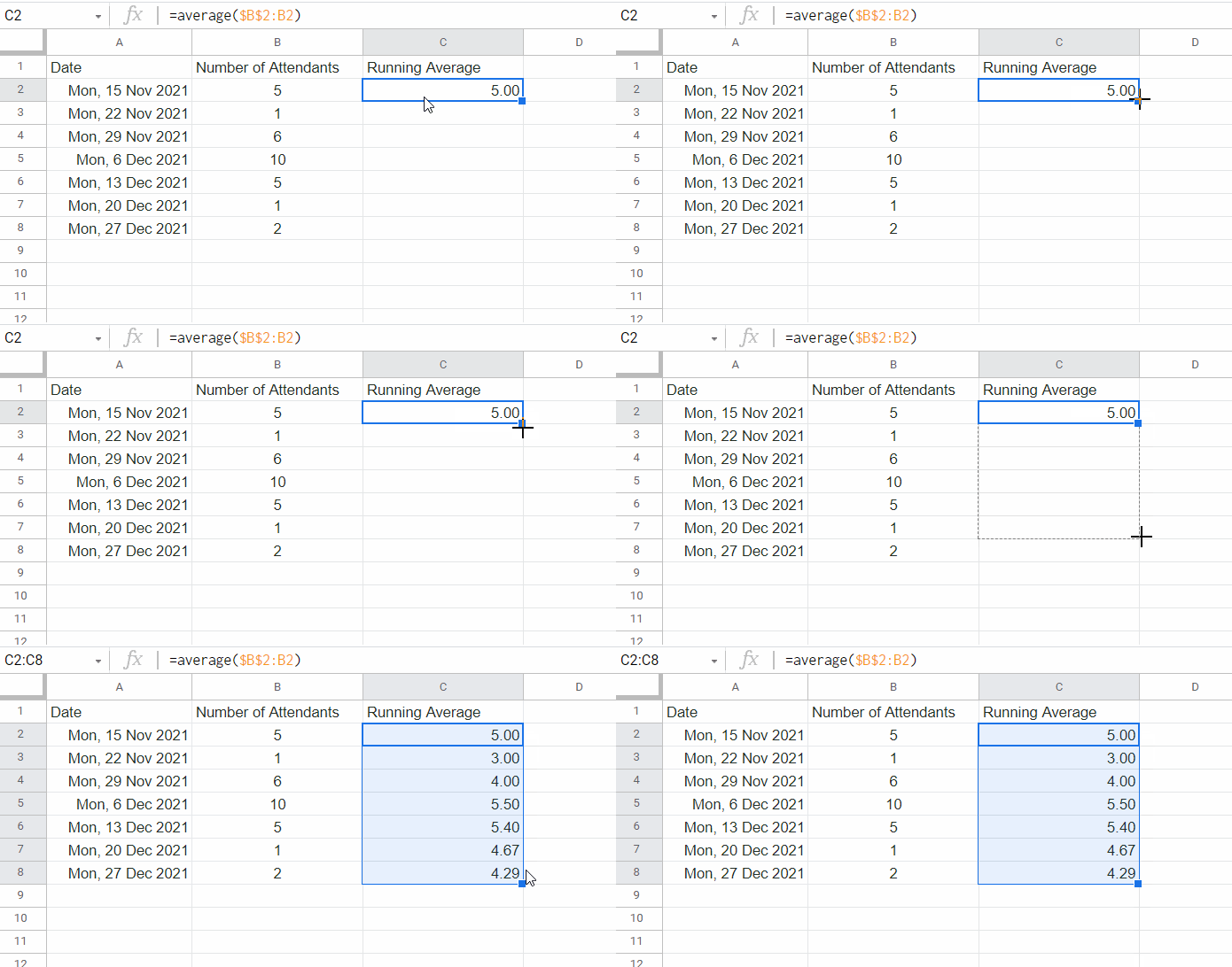
As per the following sample dataset, the dates of weekly meetings are in column A, and the number of attendants is in column B.

To calculate the running average in Google Sheets, we can use the below formula in cell C2 and copy-paste it down by dragging the fill handle as shown below.

=average($B$2:B2)

The formula will ignore any blank cell in the range B2:B8 but will count 0 (zero).

2. Running (Moving) Average Using Array Formulas in Google Sheets

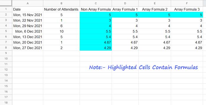
I have four running average array formula examples in Google Sheets. You won’t see the fourth one on the screenshot. It’s the Lambda formula, which I added later.

In a small dataset, all of them will work exceptionally well.

But the first and fourth running average array formulas are better at handling large datasets. It’s up to you which one to pick.

Note:- I have opened the range in all the running average array formulas. Make it closed, for example, B2:B to B2:B100, to improve their performance.

SUMIF – MA Array Formula 1

=ArrayFormula(
     if(B2:B="",,
        sumif(row(B2:B),"<="&row(B2:B),B2:B)/ifna(vlookup(row(B2:B),{filter(row(B2:B),B2:B<>""),
        sequence(counta(B2:B),1)},2,0))
     )
)

MMULT – MA Array Formula 2

=ArrayFormula(
     if(B2:B="",,
        MMULT(IF(ROW(B2:B)>=TRANSPOSE(ROW(B2:B))=TRUE,1,0),n(B2:B))/ifna(vlookup(row(B2:B),{filter(row(B2:B),B2:B<>""),
        sequence(counta(B2:B),1)},2,0))
     )
)

DAVERAGE – MA Array Formula 3

=ArrayFormula(
     if(B2:B="",,
        DAVERAGE(
           transpose({B2:B,TRANSPOSE(if(ROW(B2:B) <= TRANSPOSE(ROW(B2:B)),B2:B,))}),
           sequence(rows(B2:B),1),
           {if(,,);if(,,)}
        )
     )
)

BYROW LHF – MA Array Formula 4 (New!)

=byrow(B2:B,lambda(r,if(r="",,average(filter(B2:B,row(B2:B)<=row(r))))))

Formula Explanations

Regarding running average array formulas 1 (SUMIF) and 2 (MMULT), there are two main parts.

Part_1:

The bold part (part_1) in the formulas returns the cumulative sum of each datapoint in the range B2:B.

You can find the details under the subtitle “Array-Based Running Total Formulas in Google Sheets” in my tutorial titled Normal and Array-Based Running Total Formula in Google Sheets.

Part_2:

The second part, the sequence after the bold part_1, returns the numbers from 1 to ‘n’ and skips blank cells as detailed here – Skip Blank Rows in Sequential Numbering in Google Sheets.

While coding, I followed the below syntax.

part_1/part_2=running_average

What about Array Formula 3 (DAVERAGE)?

The DAVERAGE running average array formula is an example of how versatile Google Sheets is.

Earlier, we used database functions DMIN and DMAX to return running min and max in Google Sheets.

I have used one of those formulas here and replaced DMIN/DMAX with DAVERAGE.

Wait! I have also made one more change which is not mandatory, though.

What’s that?

The bold part in the above DAVERAGE formula for running average returns 1-12-123-1234 patterns.

I used a different formula to generate that pattern in the above referred two DMIN/DMAX tutorials.

Lambda (Array Formula 4) in Running Average:

The following FILTER will return the first value in the first row.

=filter(B2:B,row(B2:B)<=row(B2))

We must use the following formula to get the first and second values.

=filter(B2:B,row(B2:B)<=row(B3))

Using BYROW Lambda, we increment B2 to B3, B4, B5, and so on in each row.

The AVERAGE returns the mean of them in each row.

Sample_Sheet_11221

Related Resources

1. Average of Top N Percent of the Values in Google Sheets.
2. Average Array Formula Across Rows in Google Sheets.
3. Array Formula to Return Average of Every N Cells in Google Sheets.
4. How to Calculate the Simple Moving Average in Google Sheets.
5. Weighted Moving Average in Google Sheets (Formula Options).
6. Averages by Month in Google Sheets (Formula Options).
7. Average Each Row in Dynamic Range in Google Sheets.