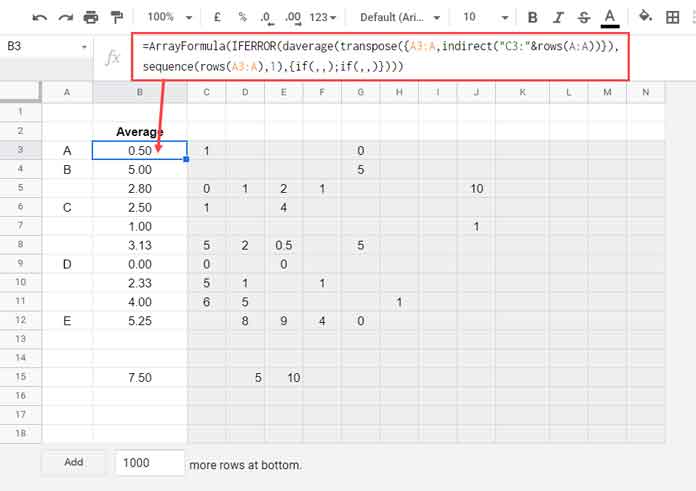
We can use the DAVERAGE function in a most unusual way to average each row in a dynamic range in Google Sheets.
The above function falls under the Database category, which usually requires structured data. But even if the data is not structured, we can use it. I’ll explain how at a later stage of this tutorial.
When it comes to getting the row-wise average, no doubt Query and MMULT are the time-tested functions to use in Google Sheets. I have already experimented with it and detailed it here – Average Array Formula Across Rows in Google Sheets.
By using DAVERAGE for getting the mean value of each row in Google Sheets, let’s be a little different from the rest of the pack.
I will show you how to use the DAVERAGE in Google Sheets to average each row in a dynamic range.
Dynamic range here means the range that is open both horizontally and vertically.
Update:- We can use BYROW() with AVERAGE() now for the same purpose! We will go to that after the DAVERAGE solution.
Average Each Row in a Dynamic Range – Using DAVERAGE
There are two main obstacles that we may face when using the DAVERAGE to get the average/mean value of each row in a dynamic range.
- It requires structured data.
- The next is not a DAVERAGE issue. It is one of the most common average problems in Spreadsheets, i.e., to skip/avoid cells containing blank or zero in the calculation.
We can address both of them.
Including Zero Values in the Dynamic Range
Formula and Example (Formula#1):
=ArrayFormula(
     IFERROR(
        daverage(
           transpose({A3:A,indirect("C3:"&rows(A:A))}),
           sequence(rows(A3:A),1),
           {if(,,);if(,,)}
        )
     )
)
The above formula is equal to using =iferror(average(C3:N3)) in B3 and drag it down until the row that you want. But here, you need to insert the formula in the top row, i.e., in cell B3. It will expand down.
The above DAVERAGE covers all the rows in the sheet from row#3 onwards and columns to its right from column C.
You can add more columns and rows to the Sheet. The formula will automatically include that rows and columns in the row-wise average calculation.
So above is one of the best ways to average each row in a dynamic range in Google Sheets.
Note:- If you face performance issues, delete unwanted/unused rows from the bottom and columns from the right.
Logic Behind the DAVERAGE Formula
Formula Syntax: DAVERAGE(database, field, criteria)
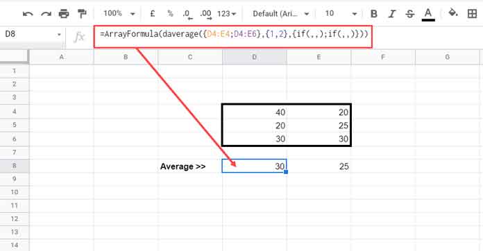
The DAVERAGE is capable of returning the average in each column in unstructured data as below.

I know I must explain it before proceeding further.
Since there are no field labels in the data range D4:E6, I used the database as {D4:E4;D4:E6} so that DAVERAGE will treat D4:E4 as the field labels.
It doesn’t matter whether D4:E4 has values or not. The DAVERAGE needs one row above the database D4:E6 to treat as field labels.
The formula returned the mean values of the columns in the database individually in D8 and E8. It is because we have specified the field as {1,2}.
The last part of the formula, i.e., {if(,,);if(,,)}, is to specify that there are no criteria to consider.
Formula Explanation
The above database function is not capable of returning the average in each row in a dynamic range. But, as you have already seen above, it works well with columns in Google Sheets.
So in our original example, we have transposed the database. The rows became columns. In that, we can apply the above logic. It’s as follows.
Database: transpose({A3:A,indirect("C3:"&rows(A:A))})
- Here
A3:Aacts as the field labels. You can use this range even if it is blank. - The formula part
indirect("C3:"&rows(A:A))is our original data range (database) and the essence of the dynamic range. For example, if you have 1000 rows in your sheet, the Indirect formula would returnC3:1000. That means all rows and columns.
Field: sequence(rows(A3:A),1)
Instead of specifying 1, 2, 3, I have automated it to cover all the rows using the Sequence function.
Criteria: {if(,,);if(,,)}
No criteria.
We can use the above formula to mean/average each row in a dynamic range, including zero in Google Sheets. The below example shows how to exclude zeros.
Excluding Zero Values in the Dynamic Range
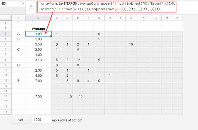
In the above same example, if you want to skip the cells containing zeros in the row-wise mean calculation, use this one.
Formula#2:
=ArrayFormula(
     IFERROR(
        daverage(
           transpose({A3:A,if(indirect("C3:"&rows(A:A))>0,
           indirect("C3:"&rows(A:A)),)}),
           sequence(rows(A3:A)),
           {if(,,);if(,,)}
        )
     )
)
The above formula is equal to using the below AVERAGEIFS in cell B3 and dragging it down.
=AVERAGEIFS(B3:N3,B3:N3,"<>0")If you compare formula#2 with formula#1, the only change is in the database part of the formula.
Here I’ve used an IF logical test to return only the values greater than zero. In other words, all the zeros are replaced by blanks.
The database functions in Google Sheets are fully flexible because we can create virtual arrays using Curly Braces and use them in it. So you may not be able to replicate the above output in Excel using the DAVERAGE.
Average Each Row in Dynamic Range – Using BYROW
Instead of DAVERAGE, we can use BYROW+AVERAGE (including zero) and BYROW+AVERAGEIF (excluding zero) to average each row in a dynamic range.
In three simple steps, I’ll help you learn how to use the above combos to average each row in a dynamic range.
We will use the same above range, i.e., C3:N18, for the calculation. Then we will see how to open it horizontally and vertically.
- To return the mean of the first row, we can use
=average(C3:N3). - We can expand this for
C3:N18using the BYROW as=iferror(byrow(C3:N18,lambda(r,average(r)))). - To open the range, replace
C3:N18withindirect("C3:"&rows(A:A))and here is that formula.
=iferror(byrow(indirect("C3:"&rows(A:A)),lambda(r,average(r))))The above is an example of the average that includes zero in each row in a dynamic range using BYROW with AVERAGE in Google Sheets.
Just replace average(r) in the formula with averageif(r,"<>0") to exclude zeros in the calculation.
=iferror(byrow(indirect("C3:"&rows(A:A)),lambda(r,averageif(r,"<>0"))))That’s all. Thanks for the stay. Enjoy!
Resources:
- Countif Across Columns Row by Row – Array Formula in Google Sheets.
- Return the First and Second Highest Values in Each Row in Google Sheets.
- Row-Wise MIN Using DMIN in Google Sheets.
- How to Use the Sumif Function Horizontally in Google Sheets.
- Column Header of Max Value in Google Sheets Using Array Formula.
- DGET Array Formula to Run Down a Column in Google Sheets.


