In this post, let’s learn how to filter rolling N days or months in Google Sheets. This means filtering a dynamic date range that adjusts based on today’s date, rather than a fixed range.
You can apply this logic to either days or months. So instead of just filtering recent days, you can also filter rolling N months in Google Sheets.
What Is a Rolling Date Range?
Rolling N days refers to the last N days relative to today—not from a fixed start date. So if today is 12-Apr-2020, a rolling 10-day window would include dates from 03-Apr-2020 to 12-Apr-2020 (inclusive). Tomorrow, the window will shift forward by one day.
That’s why it’s called rolling—the date range updates automatically as time moves forward.
Another example: If today is 31-Dec-2020, rolling 31 days would cover 01-Dec-2020 to 31-Dec-2020.
What Is a Rolling Month Range?
Rolling N months refers to the most recent completed N calendar months.
Example (as of April 12, 2020):
- Rolling 1 month = March 2020
- Rolling 3 months = Jan 2020, Feb 2020, Mar 2020
- Rolling 12 months = Apr 2019 to Mar 2020
QUERY Formula to Filter Rolling N Days in Google Sheets (30 / 90 / 120 Days)
You can use either a QUERY or FILTER formula to filter rolling N days in Google Sheets. Let’s begin with the QUERY method—especially useful if you plan to summarize the filtered data later.
Here’s a sample dataset:
| Date | Expn. | Purpose |
|---|---|---|
| 17/04/2025 | 15 | Coffee/Snacks |
| 18/04/2025 | 60 | Utilities |
| 19/04/2025 | 90 | Medical |
| 20/04/2025 | 200 | Education |
| 21/04/2025 | 500 | Childcare |
The full dataset is in the range A1:C.
Rolling 30 Days (Approx. One Month)
Paste this QUERY formula in cell E2:
=QUERY(
  A2:C,
  "SELECT *
   WHERE Col1 > date '" & TEXT(TODAY()-30, "yyyy-mm-dd") & "'
   AND Col1 <= date '" & TEXT(TODAY(), "yyyy-mm-dd") & "'",
  0
)
This will filter rolling 30 days in Google Sheets.

Tip: For more about using dates in QUERY, check out: Examples of Using Literals in QUERY in Google Sheets
Rolling 90 Days or 120 Days
Just change 30 in the above formula to 90 or 120 to filter the desired rolling window.
QUERY Formula to Filter Rolling N Months in Google Sheets (1 / 3 / 12 Months)
To filter rolling N months in Google Sheets, you’ll need a helper column to calculate the difference between each row’s month and the most recent completed month.
Step 1: Add the Helper Column
In cell D2, enter this formula:
=ArrayFormula(DATEDIF(EOMONTH(A2:A, -1)+1, EOMONTH(EDATE(TODAY(), -1), 0), "m") + 1)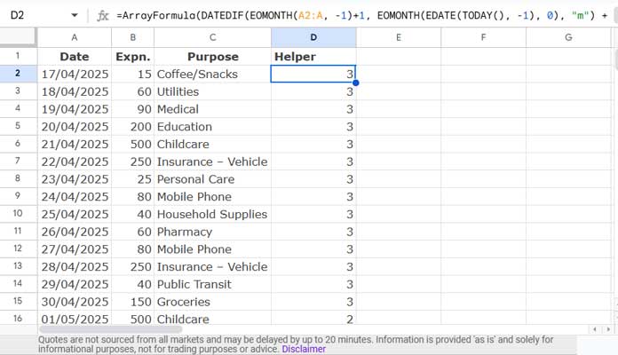
This will assign:
- 1 to the most recent completed month
- 2 to the month before that, and so on
How the Helper Column Works
EOMONTH(A2:A, -1)+1: Gives the start of the month from the date in column A.EOMONTH(EDATE(TODAY(), -1), 0): Gives the end of the most recently completed month."m": Unit for the DATEDIF function (months).
Now the dataset range becomes A2:D.
Step 2: QUERY Formula
To filter rolling 1 month in Google Sheets:
=QUERY(A2:D, "SELECT Col1, Col2, Col3 WHERE Col4 >= 1 AND Col4 <= 1", 0)In this formula, Col1, Col2, and Col3 refer to the first three columns of your dataset (e.g., Date, Expn., Purpose). You can add or remove columns in the SELECT clause based on your actual data structure.
- For rolling 3 months, change the condition to
Col4 <= 3. - For rolling 12 months, use
Col4 <= 12.
Make sure the range A2:D includes the helper column with the month offsets.
How to Omit the Helper Column
To avoid adding a physical helper column, you can build it directly inside the QUERY using HSTACK:
=QUERY(
  HSTACK(A2:C, ARRAYFORMULA(DATEDIF(EOMONTH(A2:A, -1)+1, EOMONTH(EDATE(TODAY(), -1), 0), "m") + 1)),
  "SELECT Col1, Col2, Col3 WHERE Col4 >= 1 AND Col4 <= 3",
  0
)
This will filter rolling 3 months in Google Sheets without adding a new column.
FILTER Formula to Filter Rolling 30 / 90 / 120 Days in Google Sheets
The FILTER function is even more direct for days:
=FILTER(A2:C, ISBETWEEN(A2:A, TODAY()-30, TODAY(), FALSE, TRUE))This formula will filter rolling 30 days in Google Sheets.
To adjust the rolling period, replace 30 with 60, 90, etc.
FILTER Formula to Filter Rolling 1 / 3 / 12 Months in Google Sheets
If you’ve added the helper column in column D, use:
=FILTER(A2:C, ISBETWEEN(IFERROR(D2:D), 1, 1))For rolling 3 months, use:
=FILTER(A2:C, ISBETWEEN(IFERROR(D2:D), 1, 3))To avoid the helper column:
=FILTER(A2:C, ISBETWEEN(
  IFERROR(DATEDIF(EOMONTH(A2:A, -1)+1, EOMONTH(EDATE(TODAY(), -1), 0), "m") + 1),
  1, 3
))
Note: You don’t need ARRAYFORMULA inside FILTER.
Use the Filter Menu to Filter Rolling N Days (Quick Tip)
Instead of formulas, you can use the built-in Filter Menu for quick filtering.
Steps to Apply Filter Menu for Rolling Dates
- Select the column containing the dates (e.g., Column A).
- Go to Data > Create a filter.
- Click the filter icon in the column header.
- Choose Filter by condition > Is between
- In the first box:
=TODAY()-29
In the second box:=TODAY()
This will filter rolling 30 days in Google Sheets.
Use the Filter Menu to Filter Rolling N Months (Using a Helper Column)
To filter rolling N months in Google Sheets using the Filter Menu, you must apply the filter to the helper column (e.g., Column D) that holds the month numbers.
Steps to Apply Filter Menu for Rolling Months
- Select Column D (the helper column with month numbers).
- Go to Data > Create a filter.
- Click the filter icon in cell D1.
- Choose Filter by condition > Is between.
- In the first field, enter:
1 - In the second field, enter:
N(e.g.,3for rolling 3 months,12for rolling 12 months)
This will filter rolling N months in Google Sheets, showing only the rows from the most recent N completed months.
Limitations of the Filter Menu Method
- The filter doesn’t update automatically—you must reopen the filter and click OK.
- Ensure the filter range covers all current and future data rows (check the green border).
Which Method Should You Use?
- Use QUERY if you want to both filter and summarize rolling N days or months.
- Use FILTER for quick filtering without summarization.
- Use the Filter Menu when you want to interactively sort or filter the data directly in the source.
Related Resources
- Google Sheets QUERY to Extract All Rows from Previous Month
- Filter the Last N Days of Data in Google Sheets – from today, from a specific date, or based on the latest date in the dataset
- Rolling Months Backward Summary in Google Sheets
- Rolling 7, 30, 60 Days in Pivot Table in Google Sheets
- Calculating Rolling N Period Average in Google Sheets
- Reset Rolling Averages Across Categories in Google Sheets
- Google Sheets: Rolling Average Excluding Blank Cells and Aligning


