To sum values for the current week, the first step is identifying dates that fall within the current week. Once identified, you can use various Google Sheets functions to calculate the sum. In this tutorial, you’ll learn how to accomplish this efficiently.
Your week might run from Sunday-Saturday or Monday-Sunday. The formulas provided can be adjusted accordingly.
Identify Dates in the Current Week
To find the start date of the current week, use this formula:
=TODAY()-WEEKDAY(TODAY(), 1)+1This formula considers a Sunday-Saturday week. For a Monday-Sunday week, replace the 1 in the WEEKDAY function with 2. For more details about the WEEKDAY function, refer to my guide titled Google Sheets: The Complete Guide to All Date Functions.
To determine the end date of the current week, add 6 to the start date:
=TODAY()-WEEKDAY(TODAY(), 1)+1+6Once you know the start and end dates of the current week, you can filter your data and calculate the sum for this period.
Note: You can also use the WEEKNUM function to identify the current week. However, if your dataset spans multiple years, the same week number may appear in different years, which can lead to incorrect filtering.
Sample Dataset
The dataset consists of the following columns:
- Column A: Invoice raised dates
- Column B: Invoice numbers
- Column C: Invoice amounts
The data range is A2:C, where A2:C2 contains headers. For calculations, we’ll use the range A3:C.
In cell D3, enter the formula to calculate the start date of the current week, i.e., =TODAY()-WEEKDAY(TODAY(), 1)+1.
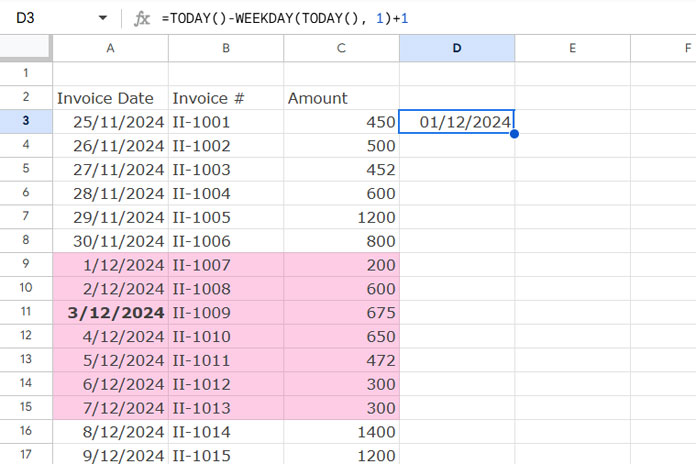
The dataset provided highlights current-week dates, assuming the current date is 2024-12-03. You can adjust the dates in Column A as needed to test the formulas effectively.
Sum Current Week’s Data in Google Sheets: Multiple Methods
Here are four methods to sum the data for the current week. Among them, SUMIF and SUMPRODUCT are the simplest.
1. SUMIF Formula
Syntax:
SUMIF(range, criterion, [sum_range])Formula:
=SUMIF(ISBETWEEN(A3:A, D3, D3+6), TRUE, C3:C)ISBETWEEN(A3:A, D3, D3+6)evaluates whether dates inA3:Afall between the start (D3) and end (D3+6) of the current week.- The criterion is
TRUE, and thesum_rangeisC3:C(invoice amounts).
2. SUMPRODUCT Formula
Syntax:
SUMPRODUCT(array1, [array2, …])Formula:
=SUMPRODUCT(ISBETWEEN(A3:A, D3, D3+6), C3:C)ISBETWEEN(A3:A, D3, D3+6)isarray1.C3:Cisarray2.- This formula multiplies matching rows and sums the result.
3. SUM + FILTER Formula
Formula:
=SUM(FILTER(C3:C, ISBETWEEN(A3:A, D3, D3+6)))- The FILTER function extracts rows from
C3:Cwhere the condition isTRUE. - SUM then calculates the total of those filtered rows.
4. QUERY Formula
Among the four formulas, this one might be slightly complex for beginners to understand because it uses a text-based query language that resembles SQL. Syntax errors can occur if column references are not specified correctly.
Formula:
=QUERY(A3:C, "SELECT SUM(C) WHERE A >=DATE '"&TEXT(D3, "YYYY-MM-DD")&"' AND A <=DATE '"&TEXT(D3+6, "YYYY-MM-DD")&"' LABEL SUM(C)''")- The QUERY function selects and sums column
CfromA3:Cwhere the dates in columnAare within the current week. TEXT(D3, "YYYY-MM-DD")formats the dates for the query.


Is there a way to make it like your post on sum by month?
Hi, Rik,
I’ll try. Can you include a link to your demo/mockup data in Google Sheets via comment? Just data in a few rows and the result you want (entered manually).
Hello,
Thank you SO MUCH for this article!!!
You say…
=filter(A3:C,weeknum(A3:A,2)=weeknum(today(),2))If I wanted to start the week on a Tuesday what would I need to change?
I tried changing 2 to 3 but I got an error.
Thank you for your help.
Hi, Terry,
The number to use to filter dates that fall on Tuesday-Wednesday is 12, not 3.
=filter(A3:C,weeknum(A3:A,12)=weeknum(today(),12))Please check WEEKNUM function in my tutorial related to Sheets Date functions.
Best,